Fractional occupation density (FOD)#

Most conventional DFT and many wave-function-theory (WFT) methods are single-reference methods and thus do not cover static electron correlation effects. Cases with strong static electron correlation typically can not be described by a single Slater determinant and are thus often referred to as "multi-reference" (MR) cases. For example, transition metal complexes and specifically those including 3d metals, are known to be prone to static electron correlation and therefore single-reference methods may not be suitable to describe them correctly. There are many MR diagnostics described in the literature with individual strengths and weaknesses. Nevertheless, the fractional occupation density (FOD) [Grimme2015] is a very simple yet powerful analytic tool to even visualize potential MR situations that is available in ORCA.

The default FOD analysis in ORCA employs the TPSS/def2-TZVP method with a electronic temperature of 5000K to "smear" static correlation prone electrons. It is simply envoked by:

!FOD

* XYZFILE 0 1 structure.xyz

Note

In principle, the FOD analysis can be performed with any functional. Nevertheless, the electronic temperature has to be adjusted to match the functional, and specifically the amount of Fock-exchange included if a hybrid is used. How to change the method and the electronic temperature is documented in the ORCA manual.

Example: Ni(bis-dithiolene)#

Let us do the FOD analysis for the potential electrocatalyst NiBDT.

!FOD

* XYZFILE 0 1 nibdt.xyz

After a successful calculation, ORCA will write the N_FOD value to the output. This value is a first indication for MR situations. In this case N_FOD is very high for a normal closed-shell complex:

N_FOD =  1.877046

Note

Note that the N_FOD value is not size-consistent and may be devided by the number of electrons if complexes of different sizes are compared.

Further, ORCA stores the FOD density in the basename.densities container which can be visualized with the orca_plot tool that is delivered with ORCA. Its interactive interface can be used via the command line input:

orca_plot basename.gbw -i

PlotType       ... MO-PLOT
MO/Operator    ... 0 0
Output file    ... (null)
Format         ... Grid3D/Binary
Resolution     ... 40 40 40
Boundaries     ...   -22.359392    16.311484 (x direction)
                     -12.628859    13.574504 (y direction)
                      -7.001812     7.002006 (z direction)

       1 - Enter type of plot
       2 - Enter no of orbital to plot
       3 - Enter operator of orbital (0=alpha,1=beta)
       4 - Enter number of grid intervals
       5 - Select output file format
       6 - Plot CIS/TD-DFT difference densities
       7 - Plot CIS/TD-DFT transition densities
       8 - Set AO(=1) vs MO(=0) to plot
       9 - List all available densities
      10 - Perform Density Algebraic Operations

      11 - Generate the plot
      12 - exit this program
Enter a number: 

Now we enter 1 to choose the type of plot we need:

-   molecular orbitals                          
-   (scf) electron density                              ......  (scfp                     )  => AVAILABLE
-   (scf) spin density                                  ......  (scfr                     )  - NOT AVAILABLE
-   natural orbitals                               
-   corresponding orbitals                         
-   atomic orbitals                                
-   mdci electron density                               ......  (mdcip                    )  - NOT AVAILABLE
-   mdci spin density                                   ......  (mdcir                    )  - NOT AVAILABLE
[...]
-   LFT QDPT unrelaxed transition AO density            ......  (Tdens-LFTQDSOC           )  - NOT AVAILABLE
Enter Type: 

Here, we choose 2 for (scf) electron density. The interface will now ask, which density should be plotted. The default electron density file is basename.scfp but as we want to plot basename.scfp_fod we change the chosen density file.

The default name of the density would be: basename.scfp
Is this the one you want (y/n)? n
Enter the FileName: basename.scfp_fod

Now, we can choose the desired output format via 5 - Select output file format, e.g., Gaussian cube, and finally generate the file basename.eldens.cube to process with the visualization program of choice via 11 - Generate the plot. To visualize the FOD, an iso surface value of 0.005 a.u. is recommended. For our example, NiBDT, the FOD plot looks like:

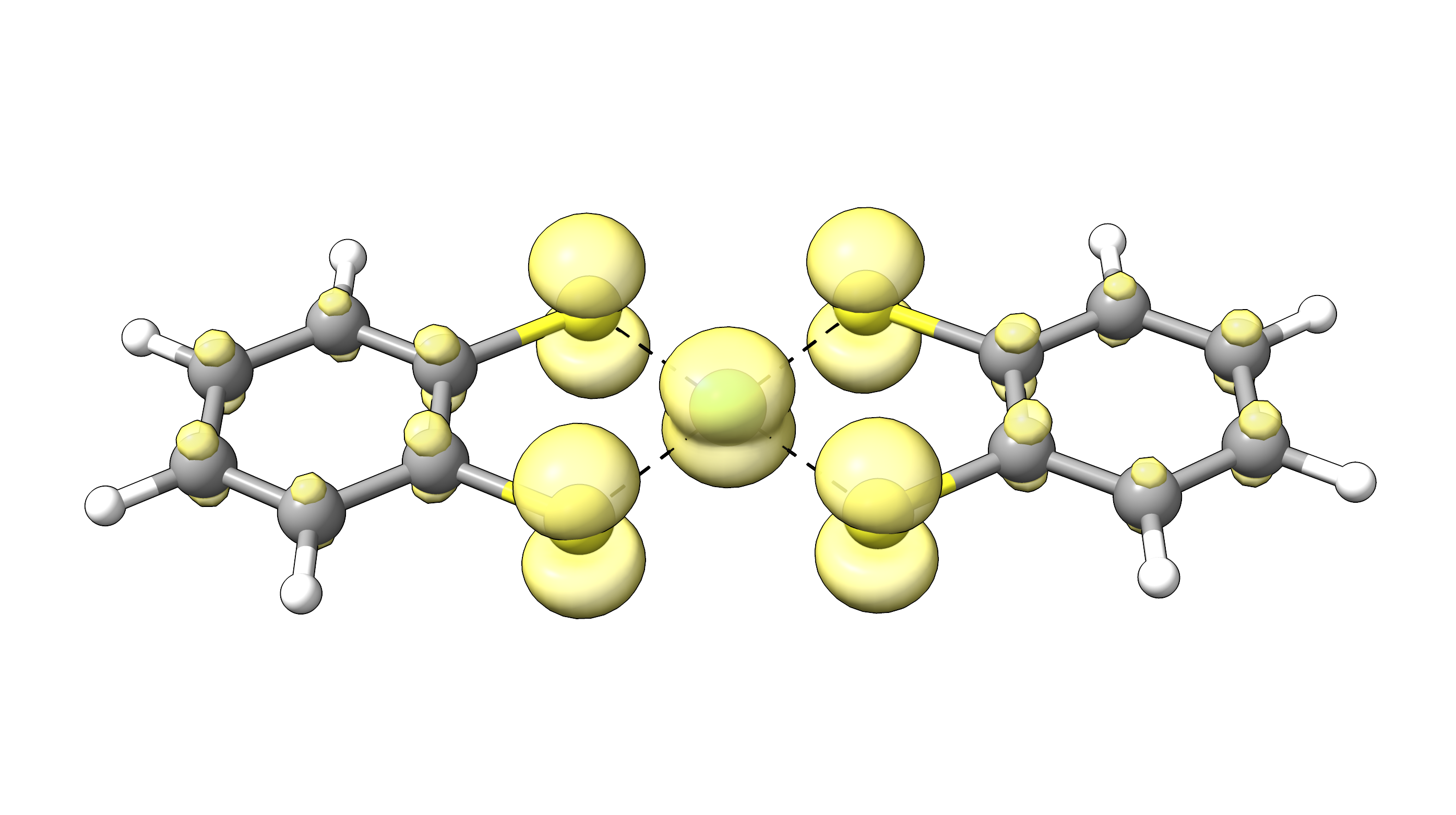
../_images/fod.png — Figure: FOD plot for NiBDT at an isosurface value of 0.005 a.u.#

The plot shows a significant delocalization of FOD over the whole molecule indicating strong static electron correlation.

For very large structures or high-throughput screening it may be further useful to use the xtb-based FOD anaylsis via ORCA. To do so, you can call xtb to do the FOD analysis via ORCAs interface to xtb:

!XTB2

%xtb
  XTBINPUTSTRING  "--fod" # string passed on to XTB call
  ETemp           5000
end

%output 
  print[p_xtb_prop] 1 
end

* XYZFILE 0 1 nibdt.xyz

For our NiBDT example, this will print the N_FOD value to the ORCA printout and will write a plottable fod.cub file in Gaussian cube format.

NFOD :     2.4882

Warning

Even though the FOD is intuitive and easy-to-use, it is not a 100% safe diagnostic for MR character and should only be used as a first indication. We recommend to always combine the FOD analysis with more sophisticated multi-reference diagnostics.

Fractional occupation density (FOD)#

Example: Ni(bis-dithiolene)#

Structures#