UVVis spectroscopy (UV/Vis)#

Predicting the UV/Vis spectrum is, essentially, predicting the electronic excited states of a system, their energies and the probabilities of transition between them.

In ORCA, there are several methods that can compute excited state properties with higher or lower accuracy, but here we will discuss only two of them: the simpler and widely used TD-DFT, that presents a good speed to accuracy trade-off, and the newer STEOM-DLPNO-CCSD, that is closer to the high-end of excited state methods.

Example: Azobenzene E/Z Isomers#

To make this rather abstract topic into something more concrete, we will try to simulate the experimental results obtained for an azobenzene derivative [Temps2009]:

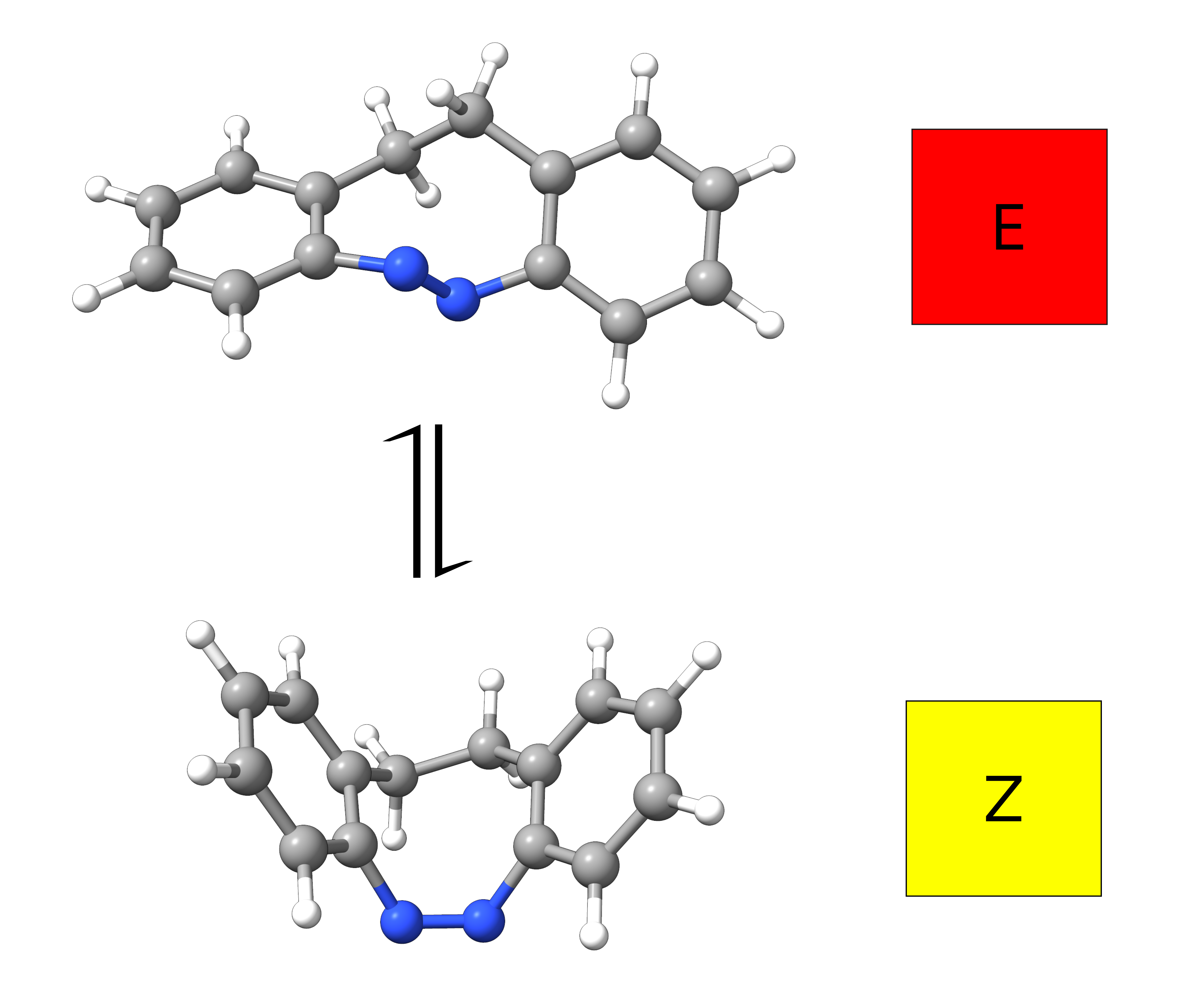
../_images/eq_color.png — Figure: E- and Z-isomer of an azobenzene derivative with their experimentally observed colors.#

It turns out that the E and Z isomers have different colors - one is yellow and the other red - and the authors attribute this to a change in the lower energy band, assigned as a \(n-\pi^*\) transition. Let's see how we could have predicted these results from first principles.

TD-DFT#

The time-dependent density functional theory (TD-DFT) is one of the most common approaches to predict UVVis spectra, because it is rather simple and not computationally too expensive. Its usage in ORCA is simple, for instance choosing the CAM-B3LYP functional and a triplet-zeta basis:

!CAM-B3LYP DEF2-TZVP CPCM(HEXANE)

%TDDFT
   NROOTS   30
END

*XYZFILE 0 1 E-isomer-optimized.xyz

The %TDDFT automatically requests the excited-state calculation necessary for the prediction of the spectrum and the NROOTS flag controls the number of excited states you want to include.

Here we also used the CPCM as a solvation model for both the ground and the excited states to simulate the hexane used in the experiment, which for the excited state case means the LR-CPCM model by default. After the regular SCF, the TD-DFT header is printed:

------------------------------------------------------------------------------
                        ORCA TD-DFT/TDA CALCULATION
------------------------------------------------------------------------------

Input orbitals are from        ... orca.gbw
CI-vector output               ... orca.cis
Solver                         ... FN-2001
Tamm-Dancoff approximation     ... operative
CIS-Integral strategy          ... AO-integrals
Integral handling              ... AO integral Direct
Max. core memory used          ... 512 MB
Reference state                ... RHF
Generation of triplets         ... off
Follow IRoot                   ... off
Number of operators            ... 1
Orbital ranges used for CIS calculation:
 Operator 0:  Orbitals  16... 54  to  55...567
XAS localization array:
 Operator 0:  Orbitals  -1... -1

with details with respect to the orbital windows, memory used and integral algorithms.

Note

The default version of TD-DFT in ORCA makes use of the TDA approximation. This can be turned off by setting TDA FALSE in the %TDDFT block.

The necessary grids are build and the Davidson procedure starts:

------------------------
DAVIDSON-DIAGONALIZATION
------------------------

Dimension of the eigenvalue problem            ...  20007
Number of roots to be determined               ...     30
Maximum size of the expansion space            ...    300
Maximum number of iterations                   ...    100
Convergence tolerance for the residual         ...    1.000e-06
Convergence tolerance for the energies         ...    1.000e-06
Orthogonality tolerance                        ...    1.000e-14
Level Shift                                    ...    0.000e+00
Constructing the preconditioner                ... o.k.
Building the initial guess                     ... o.k.
Number of trial vectors determined             ...    300


                       ****Iteration    0****
   Time for iteration     :  TOTAL=41.0 TRAFO=0.3 RIJ=2.3 COSX=22.2 XC=6.8
   Size of expansion space: 90
   Lowest Energy          :     0.098277744019
   Maximum Energy change  :     0.299673513303 (vector 29)
   Maximum residual norm  :     0.018356361086
[...]

until convergence is reached according to the tolerances printed in the header.

Finally, the converged excited states are printed:

------------------------------------
TD-DFT/TDA EXCITED STATES (SINGLETS)
------------------------------------

the weight of the individual excitations are printed if larger than 1.0e-02

STATE  1:  E=   0.093509 au      2.545 eV    20522.9 cm**-1 <S**2> =   0.000000 Mult 1
    50a ->  55a  :     0.138453 (c= -0.37209218)
    54a ->  55a  :     0.799904 (c= -0.89437354)
    54a ->  59a  :     0.027597 (c= -0.16612343)

STATE  2:  E=   0.157752 au      4.293 eV    34622.5 cm**-1 <S**2> =   0.000000 Mult 1
    45a ->  55a  :     0.010252 (c=  0.10125158)
    51a ->  55a  :     0.015135 (c= -0.12302391)
    53a ->  55a  :     0.889816 (c=  0.94330039)
    53a ->  59a  :     0.013175 (c=  0.11478184)
[...]

It is important to have in mind that these energies actually are the vertical energy differences, or the energy of that state in the ground state geometry.

Below the energies, the contributions of each single excitation are printed, first with its relative contribution (these will be discussed later), followed by the eigenvector value.

Afterwards the electronic spectrum is printed:

----------------------------------------------------------------------------------------------------
                     ABSORPTION SPECTRUM VIA TRANSITION ELECTRIC DIPOLE MOMENTS
----------------------------------------------------------------------------------------------------
     Transition      Energy     Energy  Wavelength fosc(D2)      D2        DX        DY        DZ
                      (eV)      (cm-1)    (nm)                 (au**2)    (au)      (au)      (au)
----------------------------------------------------------------------------------------------------
  0-1A  ->  1-1A    2.544515   20522.9   487.3   0.034716965   0.55690   0.74464   0.00916  -0.04823
  0-1A  ->  2-1A    4.292647   34622.5   288.8   0.015206604   0.14459  -0.00926  -0.34082  -0.16837
  0-1A  ->  3-1A    4.506793   36349.7   275.1   0.144575201   1.30939   1.14340  -0.00032  -0.04505
  0-1A  ->  4-1A    4.837811   39019.6   256.3   0.004851836   0.04094  -0.00421  -0.18168  -0.08894
  0-1A  ->  5-1A    4.869275   39273.4   254.6   0.177322389   1.48642   1.19927   0.07748  -0.20537
  0-1A  ->  6-1A    5.481984   44215.2   226.2   0.011695715   0.08708   0.01000  -0.14016   0.25949
[...]

Important

Note, that the formatting of the TD-DFT output changed with ORCA6. Please check for compatibility with any used interfaces. At this moment, the UV/Vis spectrum cannot be visualized with Avogadro.

The states and their respective vertical transition energies are printed again, now together with the oscillator strength and transition dipole moments. Strictly speaking, this is yet not a "spectrum" like the experimental one because we only have transition lines, not bands.

Plotting the calculated spectrum#

What we can do to approximate the experimental spectrum then is, e.g, convolute these lines with a Gaussian function to turn them into bands. This can be done easily by using ChimeraX using the SEQCROW plugin. Open the output file in ChimeraX, then go navigate to Tools → Quantum Chemistry → UV/Vis Spectrum. In the UV/Vis Spectrum window, you can now chose energy for weighting: electronic from the respective drop down menu and the respective plot is visualized under plot.

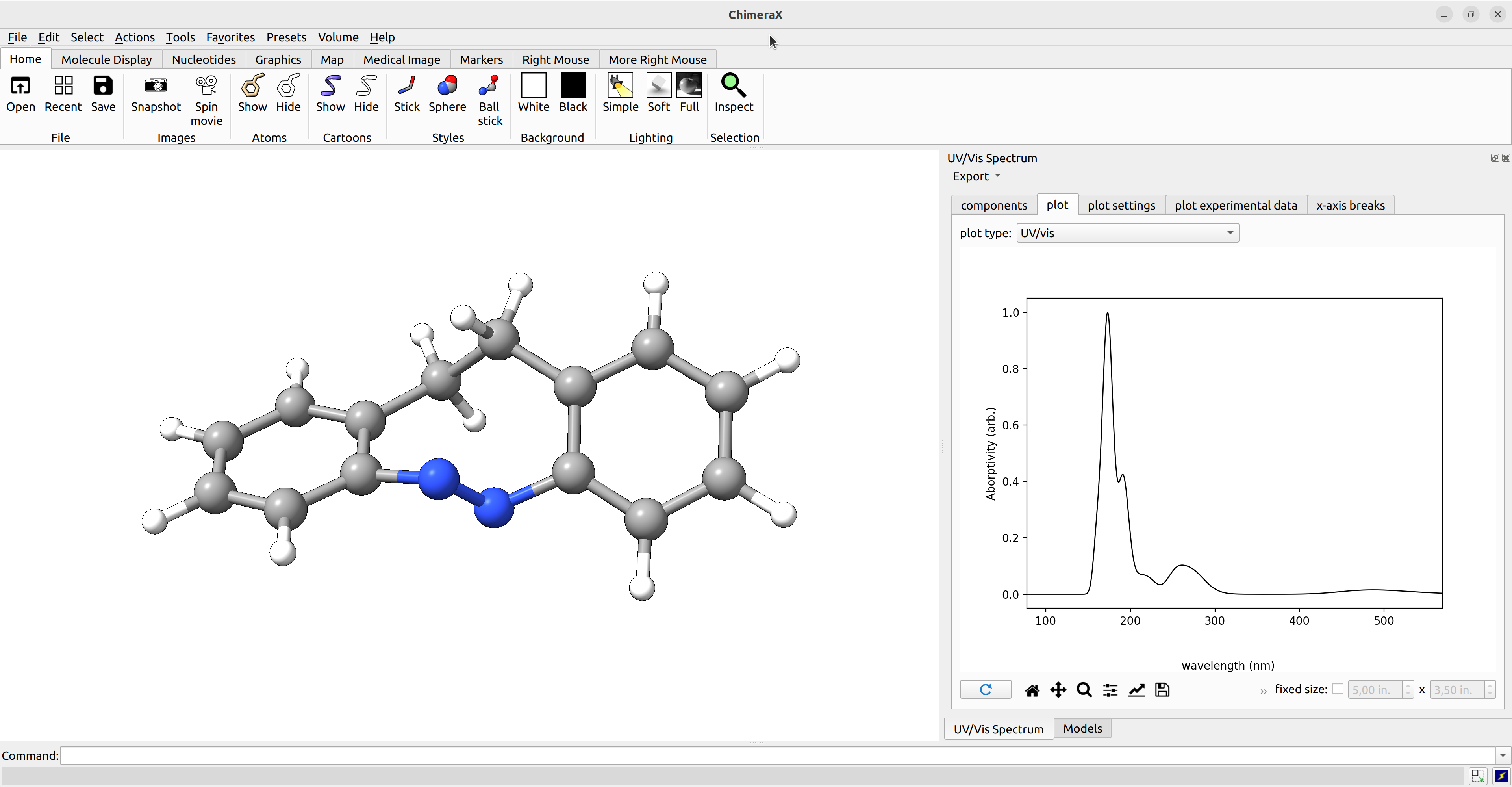
../_images/uvvis-chimerax.png — Figure: ChimeraX UV/Vis spectra panel.#

Alternatively, we can use the orca_mapspc utility program to generate plotable data from our output file. In this case we can use the following command line call:

orca_mapspc orca.out ABS -x002 -x106 -eV -n400 -w0.5

This will generate 400 datapoints from 2 to 6 eV with a Gaussian broadening of 0.5 eV. We can now plot the data with any plotting program, e.g., gnuplot.

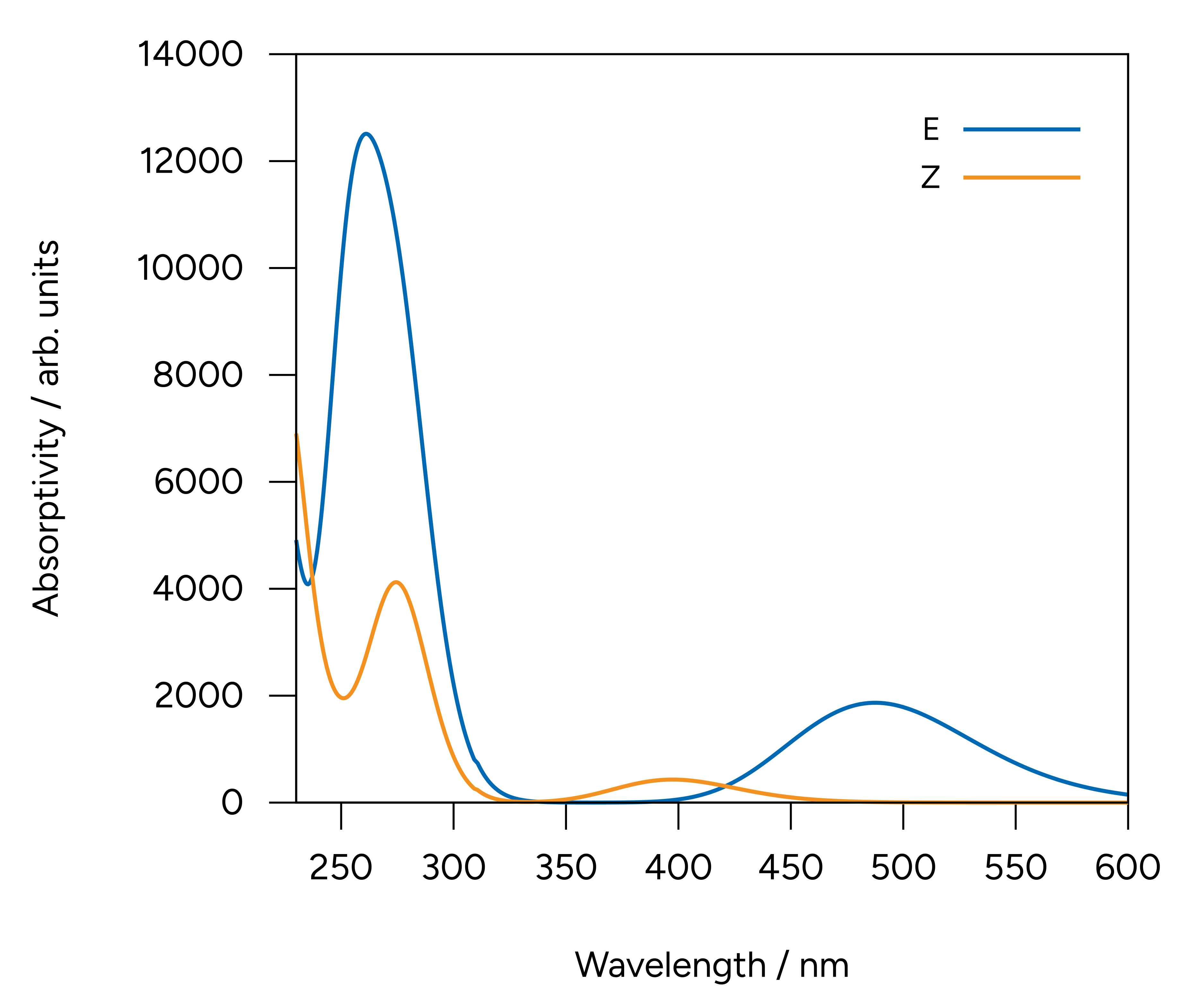
../_images/uvvis.png — Figure: Computed spectra at the CAM-B3LYP[CPCM(HEXANE)]/def2-TZVP level.#

The two low energy peaks at about 488 nm for the E and 397 nm for the Z isomer are in very good agreement with the experimental results of 490 and 404 nm, respectively. If one converts this wavelength to color and takes its complementary, the correspondence is fairly good:

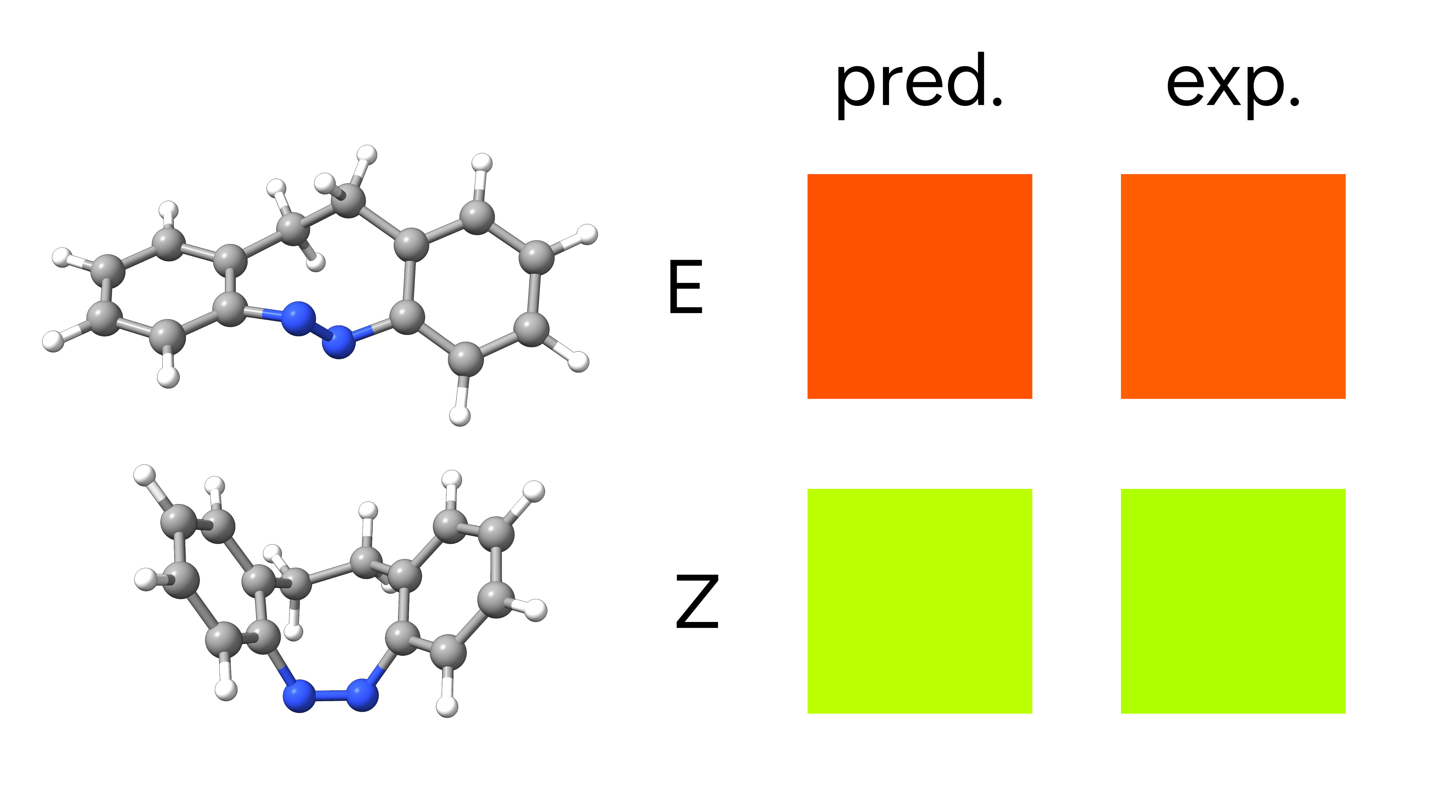
../_images/color-2.png — Figure: Complementary colors for the predicted and experimentally observed absorption maxima.#

Important

It is not that common that these results agree so well to the experiment, and here it can be somewhat accidental. It is much more prevalent that the predicted spectra is "shifted" by ±0.1 to ±0.5 eV and it is costumary in the literature to fix that, if there is any reference, to correct systematic errors.

Analysis of the Excited States#

The usual assignement for the spectral bands in azobenzenes is that the lower energy peak corresponds to the \(S_1\) state, that is of \(n\rightarrow\pi^*\) character, while the higher \(S_2\) is a \(\pi\rightarrow\pi^*\) state - which has major implications on the isomerization process.

We can make use of the calculated results to help with that complicated task, by checking on the composition of the excited states. As mentioned previously, it is printed in the TD-DFT output that the first excited state (of the E isomer) is composed of:

STATE  1:  E=   0.093509 au      2.545 eV    20522.9 cm**-1 <S**2> =   0.000000 Mult 1
    50a ->  55a  :     0.138453 (c= -0.37209218)
    54a ->  55a  :     0.799904 (c= -0.89437354)
    54a ->  59a  :     0.027597 (c= -0.16612343)

Which means that the \(S_1\) state is composed of about 80% a HOMO to LUMO transition, from orbital 54 to orbital 55 (the "a" there means alpha orbital).

If you run a calculation using LARGEPRINT on the main input, you can visualize these orbitals by opening the basename.out file directly in Avogadro 2 or ChimeraX, and they will be:

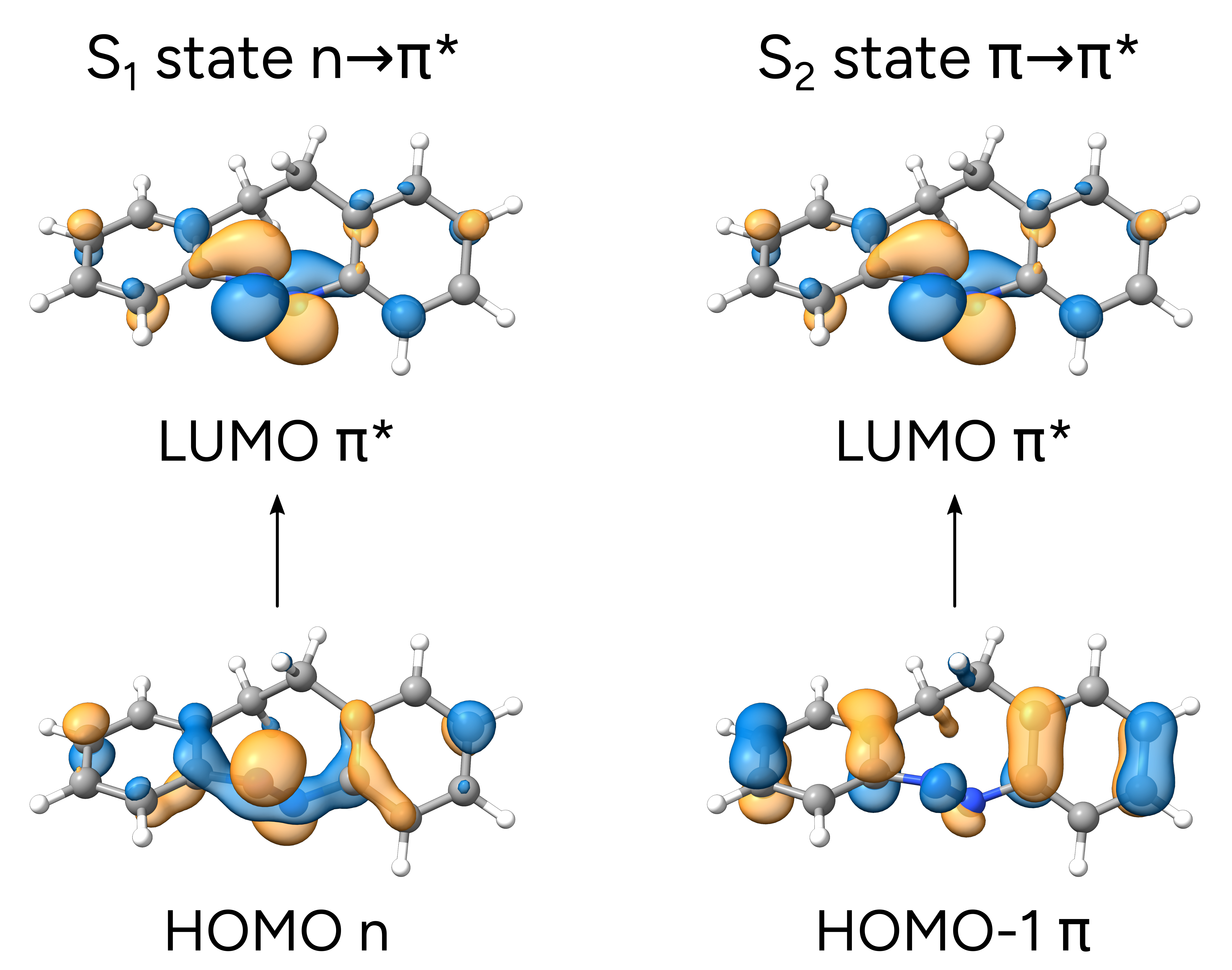
As you can see, the HOMO is a \(n\)-like molecular orbital, mostly located on the isolated electron pairs of the nitrogens, and the LUMO is a \(\pi^*\) orbital, primarily around the N=N bond, thus corroborating the suggested assignment.

We also printed the \(S_2\) main component, which is 89% HOMO-1 to LUMO transition. From the image above, it is also possible to see that the HOMO-1 now is more like a regular \(\pi\) orbital, and the \(\pi\rightarrow\pi^*\) assignment seems like a good assumption. However, now we even have the information that it is from the ring orbitals to the N=N antibonding orbital.

Important

Avogadro 2 and ChimeraX count orbitals starting from 1, but ORCA starts counting from 0. So orbital 54 in ORCA will be orbital 55 in in Avogadro 2 and ChimeraX, and so on!

Natural Transition Orbitals (NTOs)#

Another approach to investigate the nature of the excited states is to look at the NTOs of each transition [Martin2003]. These are a more compact version of the molecular orbitals and can help interpreting more complex cases. Take, for instance, the excited state 13 of the E isomer:

STATE 11:  E=   0.231920 au      6.311 eV    50900.7 cm**-1 <S**2> =   0.000000 Mult 1
    49a ->  55a  :     0.041027 (c=  0.20255160)
    50a ->  56a  :     0.175321 (c= -0.41871391)
    51a ->  58a  :     0.117541 (c= -0.34284283)
    52a ->  59a  :     0.078697 (c=  0.28052958)
    53a ->  57a  :     0.189575 (c=  0.43540185)
    54a ->  56a  :     0.193178 (c=  0.43951980)
    54a ->  59a  :     0.154964 (c=  0.39365511)

There are at least seven large transitions involved, which might be quite confusing to untangle. To evaluate the excited states in terms of their NTOs, these can be requested via DONTO TRUE in the TDDFT block:

!CAM-B3LYP DEF2-TZVP CPCM(HEXANE)

%TDDFT
   NROOTS   30
   DONTO    TRUE
END

*XYZFILE 0 1 E-isomer-optimized.xyz

The respective NTOs are now printed to the output file:

------------------------------------------
NATURAL TRANSITION ORBITALS FOR STATE   11
------------------------------------------

Making the (pseudo)densities                       ... done
Solving eigenvalue problem for the occupied space  ... done
Solving eigenvalue problem for the virtual space   ... done
Natural Transition Orbitals were saved in orca.s11.nto
Threshold for printing occupation numbers 0.001000

 E=   0.231920 au      6.311 eV    50900.7 cm**-1
    54a ->  55a  : n=  0.56085719
    53a ->  56a  : n=  0.20022822
    52a ->  57a  : n=  0.11450247
    51a ->  58a  : n=  0.08591581
    50a ->  59a  : n=  0.03500731

\(S_{11}\) is now described in terms of two dominant transitions. These NTOs are saved in a file named basename.s11.nto, and can be printed using the orca_plot tool.

After generating the .cube files for orbitals 53-56, these can be plotted using ChimeraX. To do so, simply drag-and-drop the structure .xyz and the .cube files into the ChimeraX window.

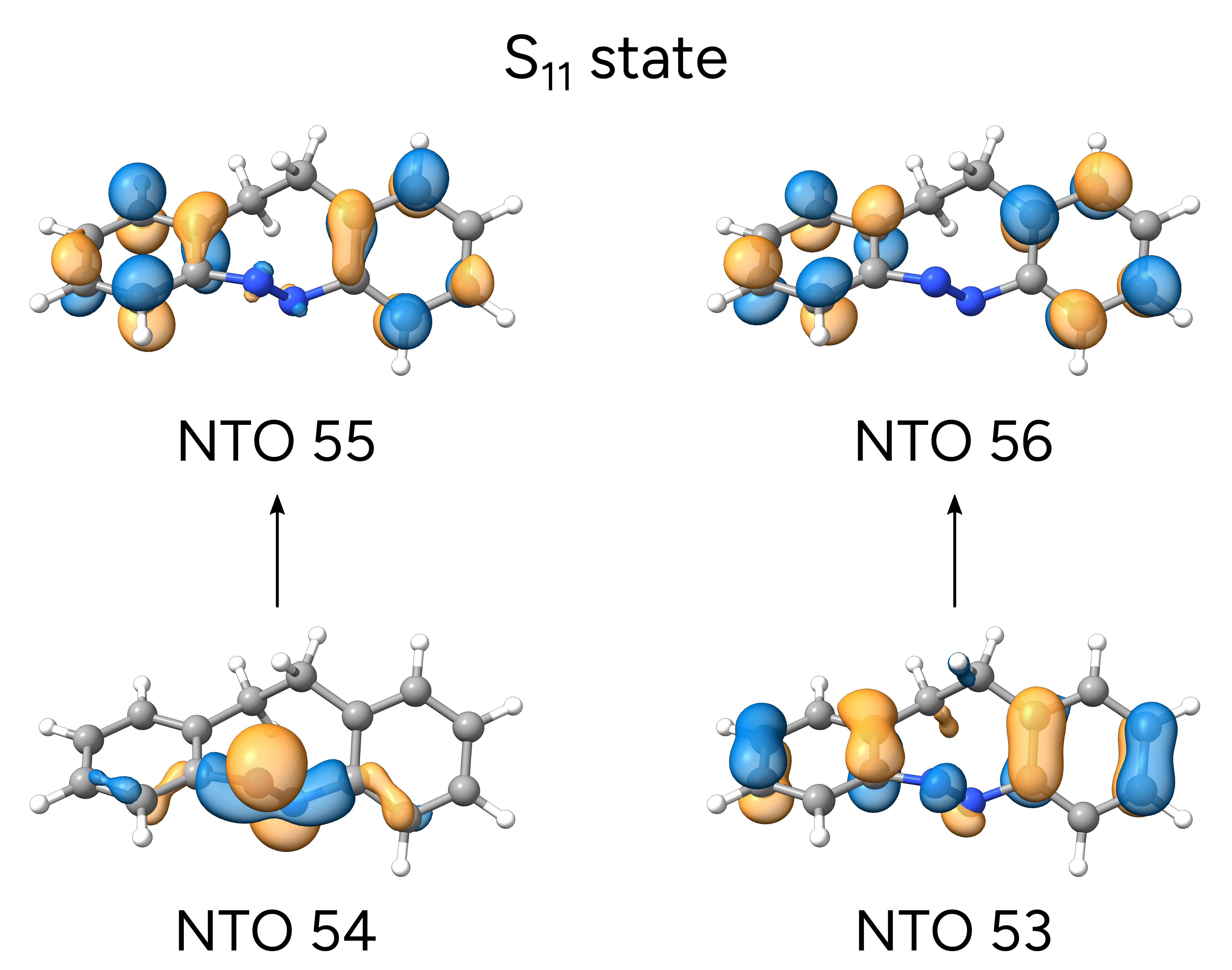
which are a dominant \(n\rightarrow\pi^*\) and aminor \(\pi\rightarrow\pi^*\) transition into the aromatic rings.

STEOM-DLPNO-CCSD#

As shown above, TD-DFT can be successful in many cases when trying to predict excited states, however one can not know a priori if a given functional will work or not and different functionals are bound to give different results.

In order to avoid this trial-and-error between functionals, an ab initio unparametrized method is sometimes a better choice. In ORCA, many of these methods are available, but for the sake of simplicity we will show here one that has a very good accuracy, still at an affordable computational cost: the Similarity Transformed Equation of Motion CCSD (STEOM-CCSD).

The STEOM-CCSD is a method that also includes Correlation energy into the calculation of the excited states, thus increasing the quality of the prediction [Iszak2019a]. It is in itself a heavy method and very computational demanding, but the ORCA team has recently developed The DLPNO scheme version of it (DLPNO-STEOM), that presents a much better scaling and it is not much costlier than TD-DFT [Iszak2019b].

In order to use that, just optimize your geometry somehow and run:

!STEOM-DLPNO-CCSD def2-TZVP def2-TZVP/C RIJCOSX CPCM(HEXANE)

%MDCI
   NROOTS  15
   DOSOLV  TRUE
END

*XYZFILE 0 1 E-isomer-optimized.xyz

As in other DLPNO or correlated methods using the RI, the /C basis is necessary for the calculation. We also added the CPCM correction for both the ground and excited states, here the latter is invoked by setting DOSOLV TRUE in the %MDCI block which controls these calcualtions.

Note

As with the other CC methods, a large amount of memory might be needed. Also, be sure you use a sufficiently large basis, of at least the size of def2-TZVP for consistent results.

The output printed is much larger than that of TD-DFT, for there are many more steps necessary to conclude the overall computation. In summary what is done is:

First a regular DLPNO-CCSD calculation is performed.

That is followed by a simple CIS calcuation, that is necessary to reduce the active space.

Then both a DLPNO-IP-EOM and a DLPNO-EA-EOM are made.

Several integrals are transformed.

Finally, the STEOM-CCSD step starts:

---------------------------------------------------
           RHF STEOM-CCSD CALCULATION
---------------------------------------------------

EOM type                                   ... STEOM
Multiplicity                               ... singlet
Solver                                     ... Davidson
Convergence check                          ... for each root separately
Convergence threshold                      ... 1.00E-05
Root homing                                ... on
Preconditioning update                     ... CIS
Reduced space size (times number of roots) ... 40
Number of roots in the CIS initial guess   ... 600
Number of roots to be optimized            ... 15
Number of amplitudes to be optimized       ... 20007
[...]

The equations are solved rootwise by default, and after everything converges, the results are printed:

------------------
STEOM-CCSD RESULTS
------------------

IROOT=  1:  0.084755 au     2.306 eV   18601.6 cm**-1
  Amplitude    Excitation
  -0.139229    49 ->  55
  -0.661523    50 ->  55
  -0.250525    50 ->  59
  -0.126564    50 ->  61
   0.110086    52 ->  55
   0.593574    54 ->  55
   0.199694    54 ->  59
  Ground state amplitude:  0.014000

Percentage Active Character     98.49

Similarly to TD-DFT, the square of the amplitudes is the percentage of that excitation in the final state. The solvent shift is done, some other integrals are calculated and the "spectrum" is printed:

----------------------------------------------------------------------------------------------------
                     ABSORPTION SPECTRUM VIA TRANSITION ELECTRIC DIPOLE MOMENTS
----------------------------------------------------------------------------------------------------
     Transition      Energy     Energy  Wavelength fosc(D2)      D2        DX        DY        DZ
                      (eV)      (cm-1)    (nm)                 (au**2)    (au)      (au)      (au)
----------------------------------------------------------------------------------------------------
  0-1A  ->  1-1A    2.284245   18423.7   542.8   0.012462857   0.22270   0.47136  -0.00551  -0.02204
  0-1A  ->  2-1A    4.254857   34317.7   291.4   0.004062678   0.03897   0.00525  -0.17419  -0.09276
  0-1A  ->  3-1A    4.356734   35139.4   284.6   0.051100120   0.47874  -0.69049  -0.00802   0.04368
  0-1A  ->  4-1A    4.730128   38151.1   262.1   0.002209585   0.01907   0.00097  -0.12248  -0.06376
  0-1A  ->  5-1A    4.862599   39219.5   255.0   0.203029647   1.70425  -1.29997  -0.03430   0.11466
  0-1A  ->  6-1A    5.431085   43804.7   228.3   0.024920419   0.18729   0.32903   0.16214  -0.22965
  0-1A  ->  7-1A    5.475070   44159.4   226.5   0.044518496   0.33189  -0.04969   0.49859   0.28430

The spectrum can be plotted using orca_mapspc as explained above:

Note

Note, that STEOM produces three separate spectra: 1. the spectrum of the right transition moments, 2. the spectrum for the left transition moments. and 3. the averaged spectrum of the left-right transition moments. The left-right spectrum should be used further. orca_mapspc will produce data for all three spectra so take care to use the correct one.

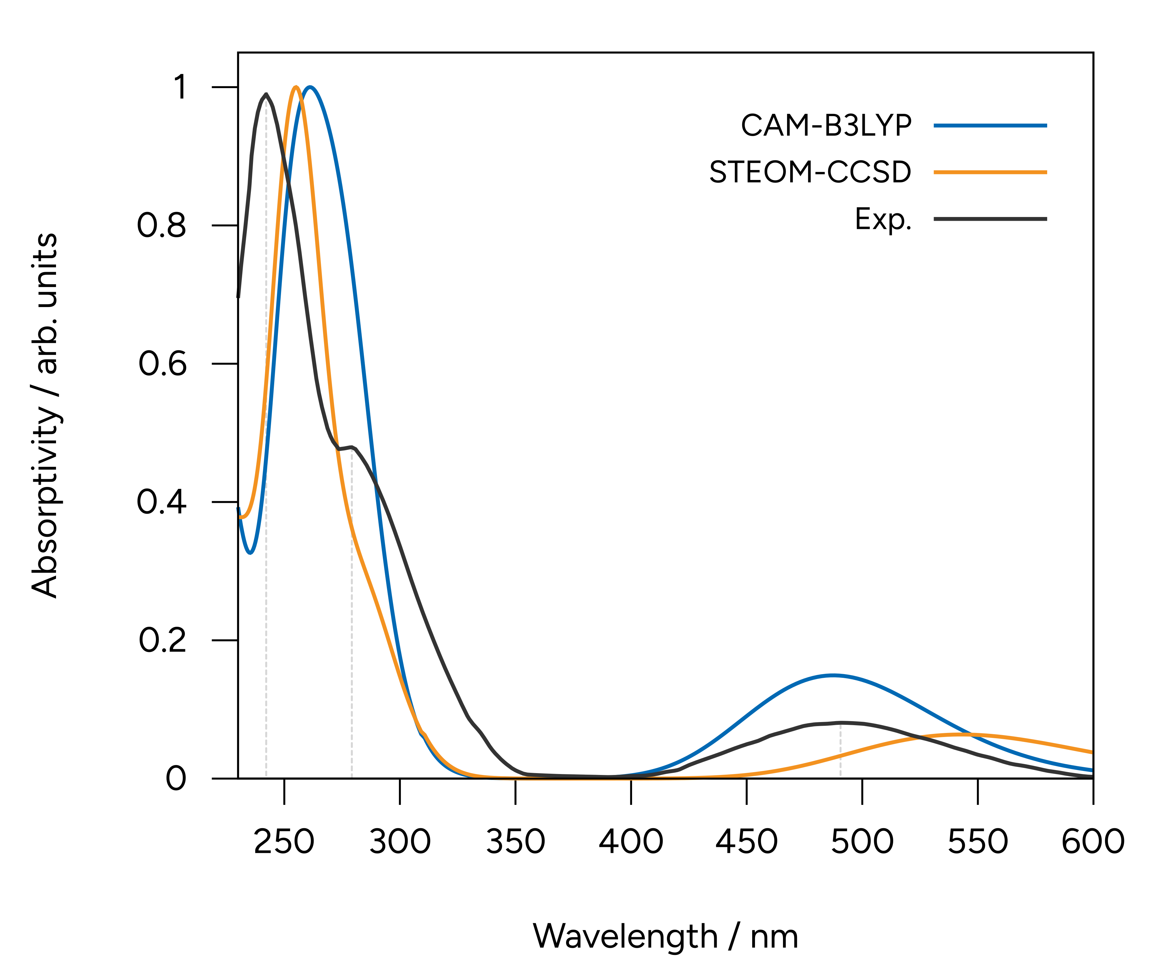
../_images/steom.png — Figure: Normalized UV/Vis spectra calculated with TD-DFT and DLPNO-STEOM-CCSD using the def2-TZVP basis set compared to the experiment.#

Here we added the gray vertical lines to guide the eye to the first three peaks of the spectrum. As you can see, although TD-DFT works well to predict the first, the higher energy ones are largely displaced.

That can happen when these states are significantly different, and the associated error is not comparable. One advantages of the STEOM is that there is a more balanced treatment of different excited states and such situations and avoided.

The calculated results are now well in line with the experiment through the whole spectrum, except for a small deviation on the relative intensities.

Important

Even if the predicted spectrum matches the experiment, the calculation is still not reproducing exactly what happens during light absorption. The full experimental spectra must also include vibrational resolution, and maybe even vibronic coupling. That can be included with the ORCA_ESD module.

UVVis spectroscopy (UV/Vis)#

Example: Azobenzene E/Z Isomers#

TD-DFT#

Plotting the calculated spectrum#

Analysis of the Excited States#

Natural Transition Orbitals (NTOs)#

STEOM-DLPNO-CCSD#

Structures#