Vibrational frequencies
After performing a Geometry optimization, you might want to compute the vibrational frequency of your system and plot normal mode animations. Here is how to do it, using the acetic acid as an example:
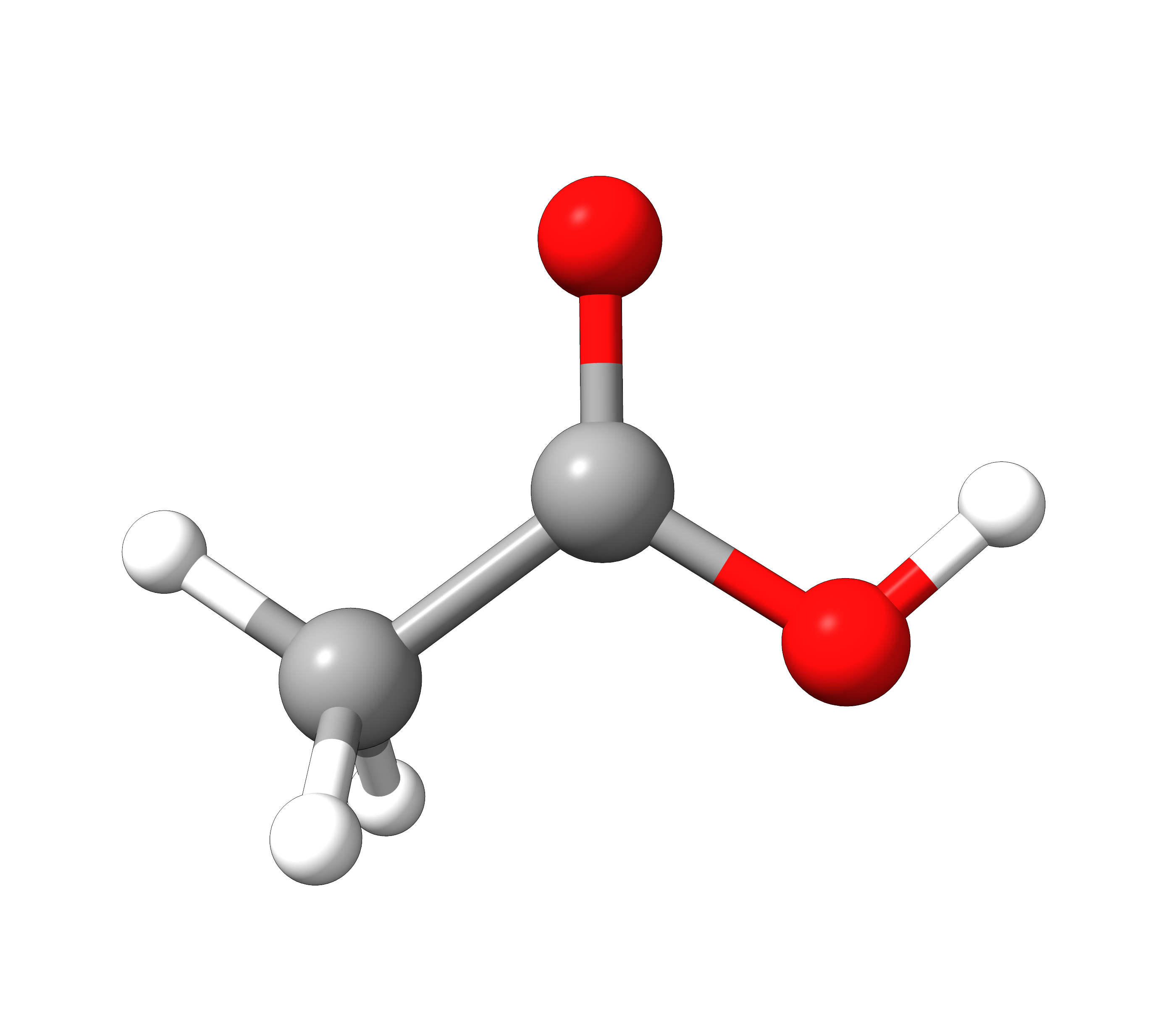
Figure: Molecular structure of acetic acid.
Frequencies
In order to first compute the frequencies, e.g. using DFT and the B3LYP functional use:
!B3LYP D4 DEF2-SVP FREQ
* XYZ 0 1
C         -0.81589       -0.51571       -0.02512
C          0.30690        0.49327       -0.06114
H         -0.42809       -1.56713       -0.28060
H         -1.26914       -0.51520        1.06962
H         -1.64631       -0.14518       -0.75104
O          0.16587        1.68279       -0.21470
O          1.51380       -0.07303        0.21899
H          2.16801        0.64625        0.13143
*
or one can also do that immediately after an optimization run using:
!B3LYP D4 DEF2-SVP OPT FREQ
* XYZFILE 0 1 aceticacid.xyz
and a geometry optimization will be performed. In case of success, it will be followed by the frequency calculation. When the computation of the Hessian matrix starts, a header will be printed:
-------------------------------------------------------------------------------
                               ORCA SCF HESSIAN
-------------------------------------------------------------------------------

Hessian of the Kohn-Sham DFT energy:
Kohn-Sham wavefunction type                      ... RKS
Hartree-Fock exchange scaling                    ...    0.200
Number of operators                              ...    1
Number of atoms                                  ...    8
Basis set dimensions                             ...   76
Integral neglect threshold                       ... 2.5e-11
Integral primitive cutoff                        ... 2.5e-12
followed by the calculation of all of the necessary terms. After it is completed, one will directly see the vibrational frequencies in \(cm^{-1}\):
-----------------------
VIBRATIONAL FREQUENCIES
-----------------------

Scaling factor for frequencies =  1.000000000  (already applied!)

0:         0.00 cm**-1
1:         0.00 cm**-1
2:         0.00 cm**-1
3:         0.00 cm**-1
4:         0.00 cm**-1
5:         0.00 cm**-1
6:        82.29 cm**-1
7:       424.53 cm**-1
8:       544.40 cm**-1
9:       593.63 cm**-1
[...]
The first few frequencies are always zero, for they correspond to the rotational and translational modes. They should be five for linear molecules and six for non-linear molecules, the rest are corresponding to actual vibrational modes.
Scaling frequencies
In case you want to multiply all your frequency values by some number after the thermodynamic functions are computed, you can use:
%FREQ SCALFREQ 1.035 END
and all frequencies would be multiplied by 1.035.
Visualizing normal modes
The vibrational modes can be animated using a suitable GUI. With Avogadro or Avogadro 2, simply open the basename.out file, and you should see a panel on the right, such as:
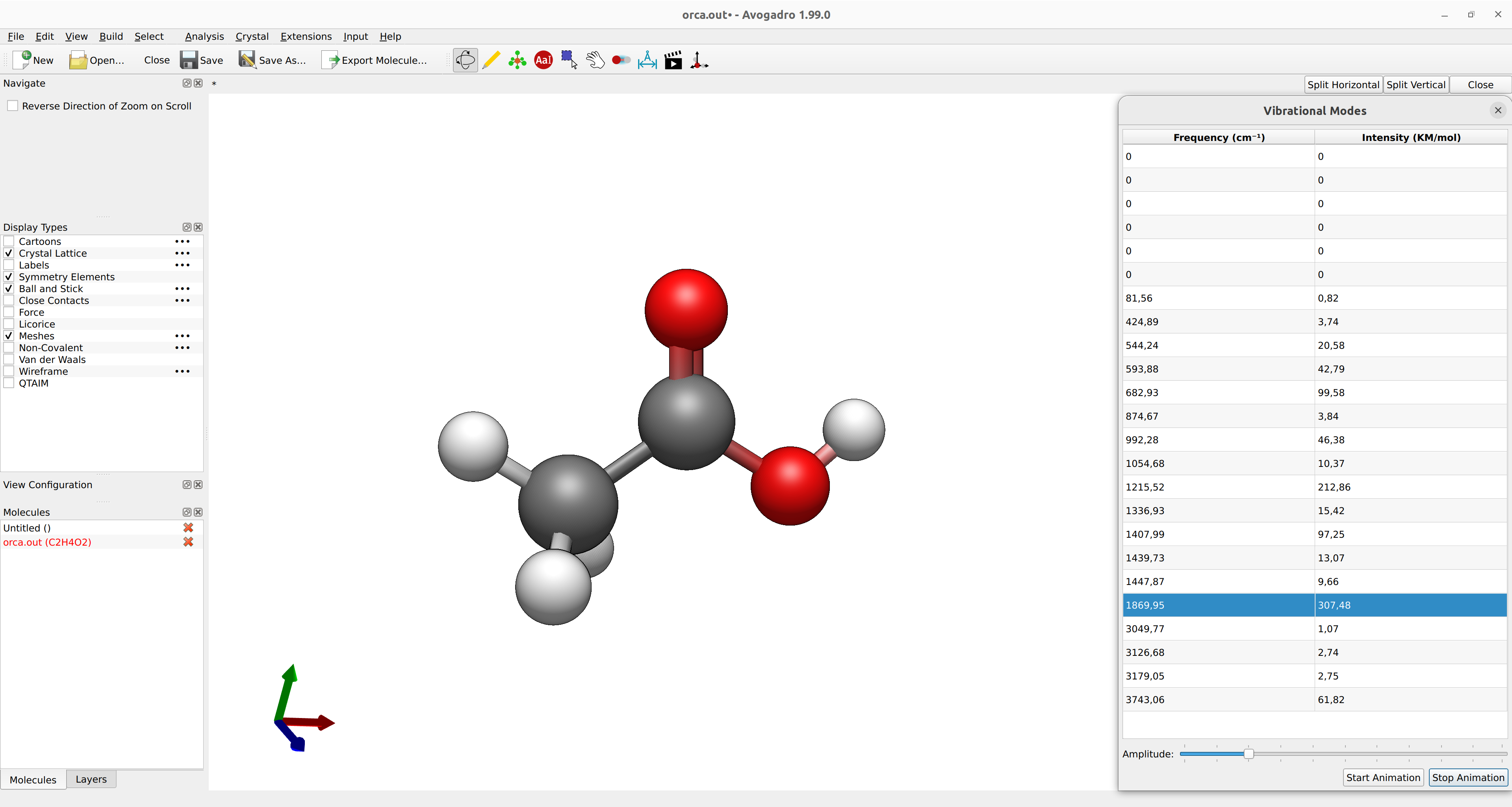
Figure: ORCA output visualized with Avogadro 2.
In ChimeraX (with SEQCROW plugin installed), you can do so as well and navigate to Tools → Quantum Chemistry → Visualize Normal Modes
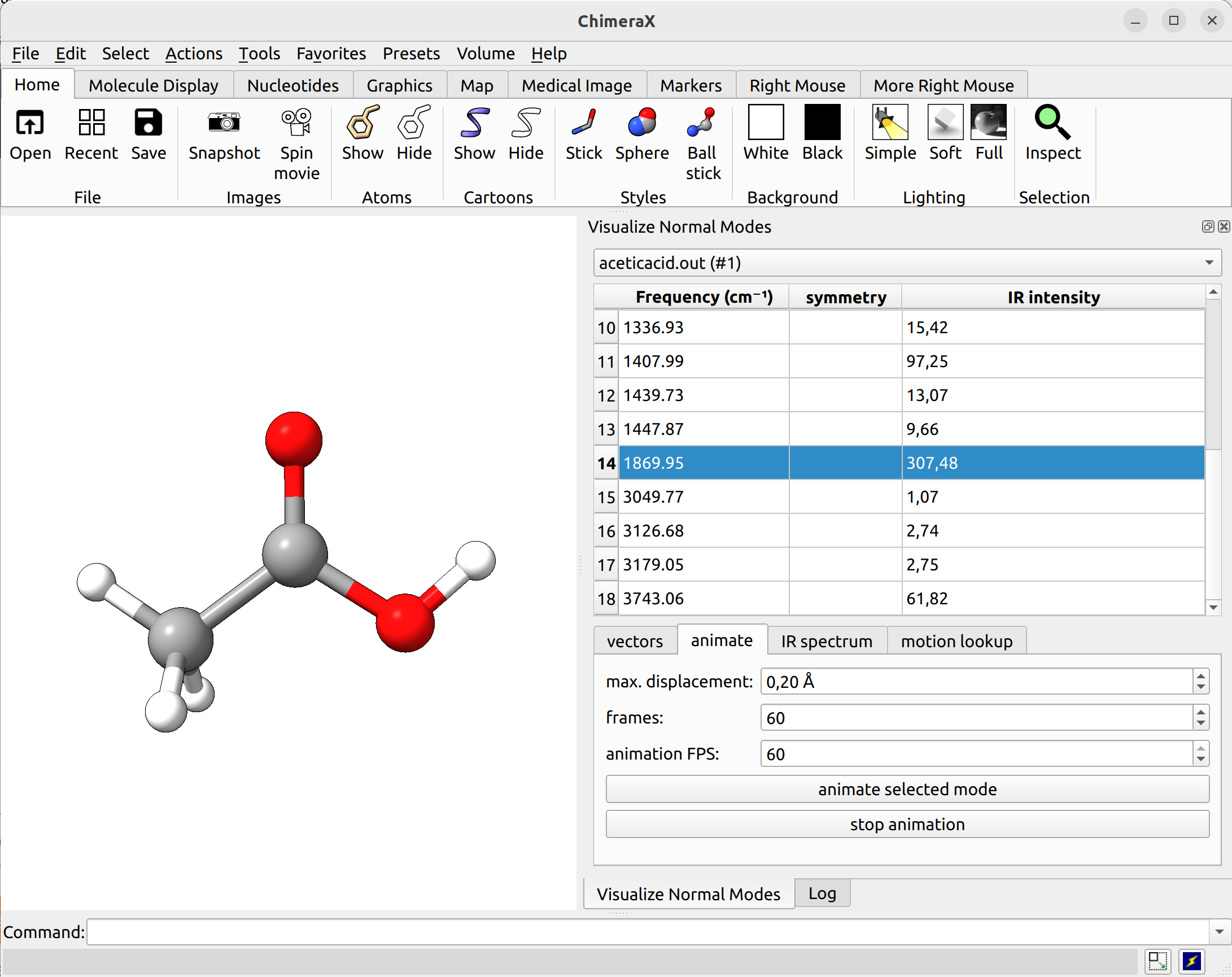
Figure: ORCA output visualized with ChimeraX.
There you can select a frequency and use the given animation option to see how exactly is the mode that corresponds to that frequency. If one clicks at the mode at about \(\sim 1800 cm^{-1}\), which is expected to be a C=O stretching mode from classical organic chemistry, one sees:
Animation: Normal mode at 1869.95 cm-1.
which corresponds to the classical prediction. The same applies for the other modes, e.g, the one at \(\sim 3150 cm^{-1}\), normally assigned as C-H stretchings:
Animation: Normal mode at 3126.68 cm-1.
Removing negative frequencies
After your calculation, if there is one or more negative frequencies, that means your structure is not a minimum on the given potential energy surface. These negative frequencies are also called imaginary modes and are specifically highlighted in the output file. Any movement along the direction of that mode reduces the energy of the molecule:
-----------------------
VIBRATIONAL FREQUENCIES
-----------------------

Scaling factor for frequencies =  1.000000000  (already applied!)

     0:       0.00 cm**-1
     1:       0.00 cm**-1
     2:       0.00 cm**-1
     3:       0.00 cm**-1
     4:       0.00 cm**-1
     5:       0.00 cm**-1
     6:     -83.22 cm**-1 ***imaginary mode***
     7:     435.79 cm**-1
     8:     544.50 cm**-1
     9:     592.38 cm**-1
Important
If possible, it is generally recommended to check your structures for imaginary modes even after an optimization run. In rare cases geometry optimizations can also converge to a non-minimum structure, e.g. a saddle-point on the potential energy surface. If your geometry is a minimum, there should be no negative frequencies. If it is a transition state, there must be only one!
In this case, the imaginary mode refers to a rotation of the methyl group.
Animation: Imaginary mode at -83.22 cm-1.
To remove such imaginary modes and converge to a minimum structure one can either try to tighten the convergence thresholds of the optimization by the TightOPT or VeryTightOPT keywords. Sometimes tightening the numerical integration grid to DEFGRID3 can also help to remove imaginary modes. If such measures fail, displacing the respective mode manually and restart the optimization can help:
!B3LYP D4 DEF2-SVP TIGHTOPT DEFGRID3 FREQ
* XYZFILE 0 1 aceticacid.xyz
Numerical Frequencies
The computation of the Hessian matrix is not available for all methods in ORCA, but one can always do a numerical Hessian calculation, using the NUMFREQ keywords, such as:
!RI-B2PLYP DEF2-SVP DEF2-SVP/C NUMFREQ
and the Hessian will be computed by the central differences approach, after \(6N\) displacements, where \(N\) is the number of atoms in your system. This can be fully parallelised and sometimes is actually a better option than the analytical FREQ calculation, depending on your memory.
Restarting NUMFREQ calculations
These calculations can take a long time if one has a large system or a heavier method. In case anything happens and the calculation ends, it can be restarted using:
!RI-B2PLYP DEF2-SVP DEF2-SVP/C NUMFREQ
%FREQ RESTART TRUE END
If the basename.hess file is present on the same folder as the input, the computation will be restarted from where stopped.
Important
There are many extra options for %FREQ, please check the ORCA manual for more info.