2. The Architecture of ORCA

In this chapter we describe the broad features of ORCA’s internal structure. This knowledge is not necessary to carry out calculations with ORCA. It may, however, help to understand which modules are being called in which order and why this is happening in the sequence it does.

2.1. The structure of the ORCA source code

The source code of ORCA is broadly structured in three parts:

1. The main program.

2. The code for the “ORCA tool library”.

3. The code for individual modules.

The code in the ORCA tool library is being compiled into one library file that subsequently is linked with all ORCA modules. The code for the individual modules can make use of everything that is in the library, but the modules are not supposed to link to or use any code of the main program or any other module. This way of structuring the code ensures that the modules remain maintainable and that there are no complex and unwanted interdependencies that would make it eventually impossible to exchange modules for new code.

2.2. The shell structure of ORCA

The whole organization of the code and the information flow can be thought of as consisting of a shell structure where a shell is a layer of software with well-defined functions and a well-defined interface to the shells above and below it.

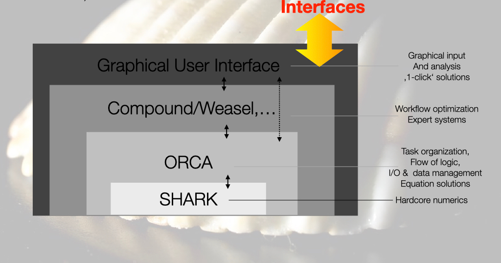
The lowest layer of the shell consists of the SHARK integral package. This is the “motor” of the program that takes care of most compute intensive tasks and essentially all parts that involve integrals over basis functions. This amounts to calculating all one- and two-electron integrals, forming Fock and Fock-like matrices and performing integral transformations using all kinds of basis sets and kernels. Most of the SHARK code is independent of the remaining ORCA source code infrastructure.

The layer above SHARK is the actual ORCA source code. ORCA interacts with the user through the interface and it orchestrates the entire workflow of the calculation. At this point in time, it also performs compute intensive tasks like forming diagonalizing and handling Fock-operators , solving large linear equation systems, forming sigma vectors, densities etc in correlated calculations and similar tasks. The ORCA source code interacts with SHARK through a small set of DRIVERS. The drivers feature genuine ORCA data structures as well as SHARK infrastructure. The DRIVERS call the genuine SHARK functions (ORCA calls SHARK directly only in a few places) and, most importantly, the DRIVERS take care of finding their way through the approximation jungle. By this we mean they handle the necessary basis sets, auxiliary basis sets, grids, integral approximations, solvation, relativity, point charges etc.

Concentrating these important and highly error prone tasks in a number of well documented routines provides a highly transparent way of identifying and properly maintaining the functionality that is at the heart of the program.

Above the ORCA software layer there are tools that orchestrate workflows. Workflows typically consisting of a number of interdepend computational steps that are later combined into a single meaningful chemical result. For example, one may optimize the geometry with a DFT functional and calculate zero-point and thermodynamic corrections at the same level and follow it up with a single point calculation at the coupled cluster level that may or may not feature another correction for core correlation at the MP2 level or complete basis set extrapolation. Such tasks and many others, like running series of calculations on a test-sets of molecules or permuting calculation options like functionals or basis sets on a given test system can be addressed with workflow tools. Inside ORCA, there is the very powerful compound scripting language to achieve and organize such tasks. On the commercial branch, FAccTs develops the Weasel tool that is a powerful and highly reliable workflow organizer.

At the final layer, one might envision a graphical user interface (GUI) that helps building molecules and facilitates running calculations and analyzing results. At this point in time, ORCA does not have a dedicated GUI. There are many free and commercial solutions that interface to ORCA. This form of interfacing is facilitated by the orca_2json interface and the property file that ORCA produces. We hope that the transparency of this interface motivates GUI developers to provide ever improved GUIs that interface ORCA. We do not exclude the possibility that ORCA will feature it’s own GUI sometime down the road.

2.3. The master/slave concept and the calling sequence

Within ORCA, the code follows a “master/slave” concept in which the main program is allowed to know everything about every module while the modules are not allowed to know anything about the main program. Thus, the main program is the piece of software that orchestrates the entire ORCA run and the interaction with the user. The main program is, however, not supposed to carry out compute intensive tasks or even parallelized tasks by itself.

An ORCA calculation commences with reading and analyzing the ORCA input file. The plausibility of this input is checked by an elaborate “maincheck” routine. Quite obviously, the number of possible combinations of ORCA features is far larger than what could possibly be checked with realistic effort. However, the maincheck routine has evolved over the year in a way that allows to detect the most common combinations of invalid or inconsistent input keywords and take appropriate action (that can be changing some parameters or aborting the job).

After through maincheck the basis sets used in the calculations and the coordinates are completely known. This is then the time to initialize the SHARK integral package and will then carry out the bulk of the computation heavy tasks.

The first module that is being called is orca_startup. This module takes care of calculating the one electron integrals such as the HCORE and overlap matrices, the metric matrices in RI calculations, the pre-screening matrices for direct SCF and possibly also the two-electron integrals for integral conventional runs.

The next module downstream is the orca_guess program. This module has the task to produce an initial set of molecular orbitals and also an initial density matrix from these orbitals. To this end, there are a number of options out of which the most common ones are to a model density guess (PMODEL) or to read orbitals from a previous calculation (MOREAD). In the latter case, the calculation may feature a different geometry and/or a different basis set but the number, nature and ordering of atoms need to be consistent with the target system.

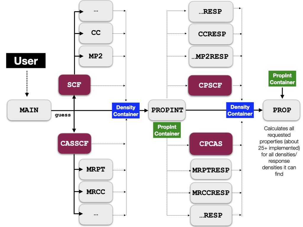
In the third step, the program branches out into either the SCF or the CASSCF module (orca_leanscf or orca_casscf). These modules produces converged orbitals and a self-consistent field energy as well as one-particle density matrix. The latter is stored in in the DensityContainer, which is a centralized storage facility for densities that will also be left over after the calculation and can be accessed by the users.

The next step of the calculation consists of calling various post-SCF programs like orca_mp2, orca_mdci or orca_autoci. NEVPT2 and CASPT2 are calculated by code that is integrated with orca_casscf. These calculate correlation energies and excited states among many other things.

There are many different pathways that the program can take next, for example geometry optimization or embedding calculations or molecular dynamics to only name a few. Rather than going into each and every one of the possible pathways, we will describe the calculation of molecular properties inside ORCA.

2.4. The calculation of molecular properties

For the calculation of molecular properties, ORCA has a fairly unique and strongly streamlined infrastructure that is focusing on the commonalities in the calculated properties and that are independent of the underlying electronic structure method used.

There are three qualitatively different sets of properties that are covered in ORCA property calculations:

1. Response properties. These are properties that can be formulated as derivatives of the total energy.

2. QDPT properties. These are properties that are calculated by quasi-degenerate perturbation theory (QDPT). This amount to diagonalizing the Hamiltonian containing external fields and relativistic corrections over a number of roots delivered by the underlying electronic structure method

3. Excited state properties: these are, at least at this point in time, transition moments between different electronic states of the system.

2.4.1. Response properties

A large number of properties can be written as derivatives of the total energy. These are first order properties:

\[X_{M}=\frac{\partial E}{\partial M}=\sum_{\mu\nu}P_{\mu\nu}^{\pm}\left\langle\mu\middle|\widehat{h}_{M}\middle|\nu\right\rangle\]

Here, \(P_{\mu\nu}^{\pm}\) is the first-order electron (‘+’) or spin (‘-‘) density \(\widehat{h}_{M}\) is the operator that is describing the property of interest (e.g. the dipole moment operator) and the basis set is \(\left\{\mu\right\}\).

Second order properties are:

\[X_{MN}=\frac{\partial^{2}E}{\partial M\partial N}=\sum_{\mu\nu}P_{\mu\nu}^{\pm}\left\langle\mu\middle|\widehat{h}_{MN}\middle|\nu\right\rangle+\sum_{\mu\nu}\frac{\partial P_{\mu\nu}^{\pm}}{\partial N}\left\langle\mu\middle|\widehat{h}_{M}\middle|\nu\right\rangle\]

Here the important quantity is \(\frac{\partial P_{\mu\nu}^{\pm}}{\partial N}\), the first derivative (or “response”) of the electron or spin density with respect to perturbation \(N\). It can be shown that the order of perturbations \(M\) and \(N\) is immaterial and hence one can choose the more convenient perturbation to calculate the response density for.

It is important to point out that the equations for response properties can always be brought into this form, irrespective of whether the calculation is a Hartree-Fock, DFT, MP2, coupled cluster, CASSCF or full-CI wavefunction.

Given the considerable generality of the property equations, it seems logical to create an infrastructure in which these similarities are exploited to the largest possible extent. In ORCA the central place where all densities and response densities are stored is the DensityContainer. This is used intensely throughout the actual calculation and left on disk as BaseName.densities where it can be used for visualization.

In terms of the calculation flow the main program contains all the logic to drive this calculation. It first drives the SCF and possibly the post-SCF calculations. After this is done, the SCF program collects the information about which property integrals will be needed down the road and call the property integral program orca_propint that will calculate the necessary integrals and stores them in another central storage container, the “property integral container”.

The next step of the calculation is that the main program determines for which properties response densities are needed. It collects these perturbations and calls the response modules. In the case of a SCF wavefunction (HF or DFT), this is the orca_scfresp program. This program will divide the requested perturbations into different types like, real-symmetric, imaginary-antisymmetric, triplet etc. Then it solves the response equations for all types of perturbations simultaneously. This leads to large efficiency gains since the same integrals are needed on the left-hand side of the coupled-perturbed SCF (CP-SCF) equations irrespective of the actual perturbations. Hence, pooling all perturbations of a given type together is much more efficient than treating these perturbations one at a time. This leads to high efficiency gains, in particular for properties like NMR parameters where nucleus dependent perturbations are required.

For a number of other electronic structure methods like MP2, CASSCF or AutoCI the respective modules can be run in “response mode” where instead of solving the equations for the energy, they pick up the amplitudes that were determined in the energy run and use them together with the property integrals in order to produce response densities.

The response densities are then stored in the density container too. At this point, one has everything that is required in order to calculate the actual properties – a task that is performed by orca_prop.

The orca_prop program works by browsing through the density container and looks for densities that are appropriate for calculating a requested property. As soon as it finds an appropriate density (or combination of unperturbed and response density), it will calculate the property. For example, if you have calculated SCF, MP2 and CCSD in the same calculation and have asked for the calculation of all three densities, orca_prop will calculate three dipole moments and print them right next to each other.

One beneficial side effect of this organization is that it is very well suited for future extensions. If a new method becomes available in ORCA that is able to produce densities and possibly response densities, the properties for this method will be fully available without any programmer needing to write a single line of additional code. It also ensures that all properties are calculated in a consistent fashion and with a consistent printout.

The results of all property calculations are stored in the central property file that will be left after the calculation. Users interested in reading properties, it should be read from the property file or its JSON translation.

2.4.2. QDPT properties

Some properties are not calculated as energy derivatives but from quasi degenerate perturbation theory. In this method one diagonalizes the QDPT matrix:

\[Q_{IJ}=\left\langle\Psi_{I}^{SM}\middle|E_{I}\delta_{IJ}+\widehat{H}_{SOC}+\widehat{H}_{SS}+\widehat{H}_{LB}+\ldots\middle|\Psi_{J}^{S'M'}\right\rangle\]

Here \(\left|\Psi_{I}^{SM}\right\rangle\) are the roots of a given method that can generate excited states with energy \(E_{I}\). For example, these can be TD-DFT roots, CASSCF roots, CASSCF roots with energy corrections from NEVPT2 or CASPT2, MRCI-roots, EOM-CCSD roots etc. and \(\widehat{H}_{SOC}\) is the spin-orbit coupling (SOC) operator, \(\widehat{H}_{SS}\) the electron-electron spin-spin coupling operator, \(\widehat{H}_{LB}\) the molecular Zeeman operator etc. In practice, only the principle component \(M=S\) (i. e. \(\Psi_{I}^{SS}\)) is calculated and the necessary matrix elements are generated using the Wigner-Eckart theorem.

The diagonalization produces the complex valued relativistic eigenstates as linear combinations of the non-relativistic or scalar relativistic eigenstates. Using the eigenstates relativistic densities or transition densities can be calculated that subsequently can be used to calculate magnetic properties or “relativistic” optical or magneto-optical spectra.

The procedure obviously suffers from a truncation error because only a finite number of roots can be calculated in practice. However, results indicate that the QDPT generated properties compare often very favorable with experimental data provided that the underlying electronic structure method delivers reasonable results.

In ORCA, all QDPT properties are calculated in a consistent infrastructure and then also leads to consistent printing and reporting of the results.

2.4.3. Excited state properties

Closely related to the QDPT infrastructure is the “one-photon absorption” (OPA) infrastructure. This is an infrastructure that coordinates the calculation of transition moments using a set of transition densities as input. These might have been stored on disk or might have been generated on the fly. In a similar way to the QDPT infrastructure, these transition moments are generated in a consistent manner throughout all modules of ORCA that can generate excited states.

The exact field/matter coupling Hamiltonian is:

\[A(\mathbf{r},t)=-A_{0}\varepsilon\exp(i\mathbf{kr}-\omega t)\]

Here \(\mathbf{k}\) is the wavevector of the radiation with frequency \(\omega\) and \(\varepsilon\) is its polarization. \(A_{0}\) is the intensity of the radiation, \(\mathbf{r}\) the electronic coordinate and \(t\) is the time.

Evaluation of the matrix element \(\left\langle\Psi_{I}^{SM}\middle|\sum_{i}{A(\mathbf{r}_{i},t)}\middle|\Psi_{J}^{S'M'}\right\rangle\) amount to generating the “exact” field-matter transition moments. This can be requested by setting the flag DoFullSemiClassical = true in the appropriate ORCA input block.

A series expansion of the cosine term yields the familiar electric dipole, electric quadrupole, magnetic dipole etc. contributions. Interestingly, the direct evaluation of the electric dipole term would yield it in the gauge independent “velocity” form. They are related to the more familiar “length” form dipole matrix elements by:

\[\left\langle\Psi_{I}^{SM}\middle|\sum_{i}\mathbf{p}_{i}\middle|\Psi_{J}^{S'M'}\right\rangle=\frac{-i}{\hslash}(E_{J}-E_{I})\left\langle\Psi_{I}^{SM}\middle|\sum_{i}\mathbf{r}_{i}\middle|\Psi_{J}^{S'M'}\right\rangle\]

The results of the length and velocity transition moment evaluation are expected to match in the basis set limit if the electronic structure method at hand satisfies certain conditions. In practice, they usually do not agree very well, even if large basis sets are used.

In order to generate electric length and velocity as well as higher moment evaluations, you can use the keywords

DoDipoleLength   = true
DoDipoleVelocity = true
DoHigherMoments  = true

in the appropriate ORCA input blocks that trigger the respective excited state calculation.