7.17. Interface to SINGLE_ANISO module
7.17.1. General description
The SINGLE_ANISO program allows the non-perturbative calculation of
effective spin (pseudospin) Hamiltonians and static magnetic properties
of mononuclear complexes and fragments on the basis of an ab initio,
including the spin-orbit interaction. As a starting point it uses the
results of a CASSCF/NEVPT2/SOC calculation for the ground and several
excited spin-orbit multiplets.
The following quantities can be computed:
Parameters of pseudospin magnetic Hamiltonians (the methodology is described in [168]) :
First order (linear after pseudospin) Zeeman splitting tensor (\(g\) tensor), including the determination of the sign of the product \(g_X\cdot g_Y\cdot g_Z\).
Second order (bilinear after pseudospin) zero-field splitting tensor (\(D\) tensor).
Higher order zero-field splitting tensors \((D^2, D^4, D^6, ..., etc.)\)
Higher order Zeeman splitting tensors \((G^1, G^3, G^5, ..., etc.)\)
Crystal-Field parameters for the ground atomic \(\tilde{J}\) multiplet for lanthanides. [414, 859]
Crystal-Field parameters for the ground atomic \(\tilde{L}\) term for lanthanides and transition metals.
Static magnetic properties [857, 858]:
Van Vleck susceptibility tensor \(\chi_{\alpha\beta}(T)\).
Powder magnetic susceptibility function \(\chi(T)\).
Magnetisation vector \(\vec M(\vec H)\) for specified directions of the applied magnetic field \(\vec H\).
Powder magnetisation \(\overline{M_{mol} }(H,T)\).
Magnetisation torque function \(\vec{\tau}_{mol}(H,T)\).
The magnetic Hamiltonians are defined for a desired group of \(N\)
low-lying electronic states obtained in CASSCF/SOC calculation to
which a pseudospin \(\tilde{S}\) is subscribed according to the relation
\(N=2\tilde{S}+1\). The pseudospin \(\tilde{S}\) reduces to a true spin
\(S\) in the absence of spin-orbit coupling. For instance, the two wave
functions of a Kramers doublet correspond to the pseudospin
\(\tilde{S}=1/2\). The implementation is done for \(any\) dimension of the
pseudospin \(\tilde{S}\), and controlled by the keyword MLTP.
The calculation of magnetic properties takes into account the
contribution of excited states (the ligand-field and charge transfer
states of the complex or mononuclear fragment which were included in the
CASSCF/CASPT2 calculation) via their thermal population and Zeeman
admixture. The effect of intermolecular exchange interaction between
magnetic molecules on the resulting magnetic properties in a crystal is
described by a phenomenological parameter \(zJ\) specified by the user.
7.17.2. Running SINGLE_ANISO calculations
The SINGLE_ANISO is, in principle, a stand-alone utility
(otool_single_aniso) that can be called directly from the shell with
its own input file, provided that the ab initio datafile is available:
bash:$
bash:$  $ORCA/x86_64/otool_single_aniso < single_aniso.input > single_aniso.output
bash:$
However, this usage may not be so convenient, as the file
single_aniso.input must include the true name of the datafile. For the
user’s convenience, a deeper integration between SINGLE_ANISO and
CASSCF program in ORCA was implemented, as described below.
As a prerequisite for using the SINGLE_ANISO module to calculate the
magnetic properties of the investigated compound, spin-orbit coupling
and other relativistic effects are already taken fully into account at
the stage of quantum chemistry calculation of the investigated
compound. The necessary information of the ab initio calculation is
provided in a form of a “datafile”: energy spectra, angular momentum
integrals, etc. The interface with ORCA generates the required
datafile automatically. The following naming conventions were adopted
for the datafile in function of the employed computational method:
CASSCF+SOC+SINGLE_ANISO\(=>\)"$orca_input_name.CASSCF.anisofile"CASSCF+QD-NEVPT2+SOC+SINGLE_ANISO\(=>\)"$orca_input_name.NEVPT2.anisofile"
Note that if the CASSCF+QD-NEVPT2+SOC+SINGLE_ANISO calculation is
requested, then the SINGLE_ANISO will be executed twice, and the above
two datafiles will be generated. The interface will generate the
SINGLE_ANISO input file with the keywords information provided in the
CASSCF/aniso subblock. These filename of the datafile is included
automatically in the input file for the SINGLE_ANISO utility (keyword
DATA), also generated automatically by the interface. The naming
convention for the generated input files for the SINGLE_ANISO utility
is “$orca_input_name.anisofile”.
All keywords of the SINGLE_ANISO program are possible to be specified
within the CASSCF/ANISO subblock. They are referenced in Section
Reference list of CASSCF/ANISO keywords. Optionally, a working
SINGLE_ANISO input file can be passed directly to the CASSCF module
setting the filename with keyword InputNameOnDisk in the ANISO
subblock.
An example of the full ORCA input for performing magnetic properties
calculations within the CASSCF/SOC/SINGLE_ANISO methodology for a
hypothetical Co(II) compound is provided below:
! 6-31G TightSCF   # basis set and other global ORCA settings

%maxcore 2000

%casscf nel 7
  norb 5           # 7 electrons in 5 orbitals (3d shell)
  mult 4, 2
  nroots 10, 40     # 10 quartet and 40 doublet states

  rel
  dosoc true       # include spin-orbit coupling
  end

  ANISO
    doaniso true     # generate datafile/input and call
                     # the SINGLE_ANISO module
    MLTP 2,2,2,2     # group of spin-orbit states for which the pseudospin
                     # Hamiltonian is computed: 4 low-lying spin-orbit doublet states.

    TINT 0, 300, 301 # 301 steps in the temperature interval [0-300]
                     # for magnetic susceptibility (in Kelvin)
    HINT 0, 7.0, 71  # 71 steps in the field interval [0-7]
                     # for molar magnetisation (in Tesla)
    TMAG 1.0,1.2,1.8,2.5,3.6  # temperature points for which molar magnetisation
                                              # is computed
     CRYS_element "Co"
     CRYS_charge 2
     PLOT true         # requires the ANISO to produce gnuplot scripts,
                              # datafiles and plots of various quantities

    # Alternative to the snippet above. Provide separate input file:
    # InputFile "$orca_input_name.anisoinput"
  end
end

*xyz 0 4   # charge is 0 for this neutral compound
Co   -2.80118000    9.91634000   19.40386000
O    -3.59660000   12.00284000   20.51731000
O    -5.12835000   10.85934000   19.53431000
O    -5.70975000   12.39302000   20.99406000
O    -1.30202341   11.67611386   19.17300658
O    -3.84191000    9.45315000   21.48634000
O    -1.27500262    8.12582233   19.18634310
O    -3.94611990    9.65426823   17.48476360
N    -4.85020000   11.78071000   20.36823000
H    -1.23636310   12.09677337   18.41017549
H    -1.07910455    7.59540828   19.85227241
H    -3.30514987    9.28034259   22.26327382
H    -4.79957696    9.43862752   21.55163236
H    -4.64801074    9.00163025   17.42987361
H    -3.73273676   10.19508893   16.72083912
H    -0.75470916   11.94100908   19.91589125
*
The input above utilises the following keywords: MLTP keyword requires
the computation of the \(g\) tensor for 4 groups of spin-orbit states, the
dimensionality of each group being 2 (Kramers or Ising doublets). TINT
requires computation of the magnetic susceptibility in the temperature
interval 0 K - 300 K distributed equally in 300 temperature intervals.
TMAG requires computation of powder molar magnetisation at 6
temperature points, in Kelvin (K): 1.0 K, 1.2 K, 1.8 K, 2.5 K, 2.9 K and
3.6 K. HINT defines the range for the magnetic field strength, in
Tesla. PLOT keyword invokes the plotting function of the module.
CRYS_element + CRYS_charge request for the computation of the crystal
field parameters for the ground term of the Co\(^{2+}\) ion. For more
information about the keywords in SINGLE_ANISO module, you can refer
to section
Reference list of CASSCF/ANISO keywords.
Please always check the obtained orbitals after CASSCF
calculation. In this particular case, the active orbitals (45-49) are
localised on the Co site and display dominant 3\(d\) character.
                45        46        47        48        49
           -0.37264  -0.36672  -0.36520  -0.36153  -0.35018
            1.40513   1.40270   1.39998   1.39823   1.39395
            --------  --------  --------  --------  --------
0 Co s         0.0       0.0       0.0       0.0       0.2
0 Co pz        0.1       0.1       0.1       0.0       0.0
0 Co px        0.0       0.2       0.0       0.0       0.1
0 Co py        0.1       0.1       0.0       0.0       0.1
0 Co dz2      23.6      39.5      10.0       2.0      23.5
0 Co dxz      12.8      30.8      48.6       4.4       2.2
0 Co dyz      46.5      10.4      19.3      20.8       2.4
0 Co dx2y2     6.9       0.3      21.2      69.2       1.6
0 Co dxy       9.5      17.6       0.2       2.8      68.0
We see that in the above output section, the five active orbitals have dominant contribution from the Co-3\(d\) basis functions. This is OK and is expected for common transition metal compounds. For lanthanide compounds, the seven active orbitals should have dominant contribution from the 4\(f\) shell. Larger active spaces must be carefully inspected and analysed. We refer here to the respective section of this manual describing the CASSCF method and how to achieve convergence The Complete Active Space Self-Consistent Field (CASSCF) Module.
The results calculated by using SINGLE_ANISO module are placed after
the SOC section in ORCA output. Here is the explanation for these
results.
%%%%%%%%%%%%%%%%%%%%%%%%%%%%%%%%%%%%%%%%%%%%%%%%%%%%%%%%%%%%%%%%%%%%%%%
CALCULATION OF PSEUDOSPIN HAMILTONIAN TENSORS FOR THE MULTIPLET 1 ( effective S =  1/2)
%%%%%%%%%%%%%%%%%%%%%%%%%%%%%%%%%%%%%%%%%%%%%%%%%%%%%%%%%%%%%%%%%%%%%%%
The pseudospin is defined in the basis of the following spin-orbit states:
spin-orbit state 1. energy(1) =       0.000 cm-1.
spin-orbit state 2. energy(2) =       0.000 cm-1.

g TENSOR:
|--------------------------------------------------------|
|    MAIN VALUES    |             MAIN MAGNETIC AXES     |  x , y , z  -- initial Cartesian axes
|-------------------|----|----- x ------- y ------- z ---|  Xm, Ym, Zm -- main magnetic axes
| gX =   0.09871069 | Xm | -0.456536 -0.363638  0.811998 |
| gY =   0.11729280 | Ym |  0.643532  0.495246  0.583605 |
| gZ =  11.21949040 | Zm | -0.614361  0.788985  0.007914 |
|--------------------------------------------------------|
The sign of the product gX * gY * gZ for multiplet 1: < 0.
The section above shows the \(g\) tensor for the ground Kramers doublet. Since the \(g_X\) and \(g_Y\) are much smaller than the \(g_Z\) component, the \(Zm\) axis is denoted as the \(main magnetic axis\) of the computed molecule. The “Zm \(|\) -0.614361 0.788985 0.007914 \(|\)” denotes the Cartesian components of the \(Zm\) vector.
In the case the computation of the parameters of the crystal field is
requested by CRYS_element and CRYS_charge, the following section
will be found in the output:
%%%%%%%%%%%%%%%%%%%%%%%%%%%%%%%%%%%%%%%%%%%%%%%%%%%%%%%%%%%%%%%%%%%%%%%
     CALCULATION OF CRYSTAL-FIELD PARAMETERS OF THE GROUND ATOMIC TERM, L =  3.
%%%%%%%%%%%%%%%%%%%%%%%%%%%%%%%%%%%%%%%%%%%%%%%%%%%%%%%%%%%%%%%%%%%%%%%

The parameters of the Crystal Field matrix are written in the coordinate system:
(Xm, Ym, Zm) --  the main magnetic axes of the ground pseudo-L = | 3> orbital multiplet.
Rotation matrix from the initial coordinate system to the employed coordinate system is:
-------------------------------------------------------------------|
x , y , z  -- initial Cartesian axes                               |
Xm, Ym, Zm -- main magnetic axes                                   |
                     x                 y                 z         |
      | Xm | -0.61155332461133 -0.79120321735748  0.00000000001900 |
 R =  | Ym |  0.79120321735748 -0.61155332461133 -0.00000000000264 |
      | Zm |  0.00000000001371  0.00000000001342  1.00000000000000 |
-------------------------------------------------------------------|
Quantization axis is Zm.


----------------------------------------------------------------------------------------------|
   Ab Initio Crystal-Field Splitting Matrix written in the basis of Pseudo-L Eigenfunctions   |
----------------------------------------------------------------------------------------------|
          |                    | -3 >               |                    | -2 >               |
----------|---------- REAL ----------- IMAGINARY ---|---------- REAL ----------- IMAGINARY ---|
   < -3 | |  -777.2218617165776     0.0000000000000 |    -0.0000000454613     0.0000000351393 |
   < -2 | |    -0.0000000454613    -0.0000000351393 |   285.4563720817839     0.0000000000000 |
   < -1 | |     0.0285952366255    -0.0055088548681 |     0.0000000002580    -0.0000000024089 |
   <  0 | |    -0.0000000160911     0.0000000604843 |     0.0001933353720    -0.0013498718536 |
   <  1 | |     0.0116130821579    -0.0096419531309 |    -0.0000000005651    -0.0000000026613 |
   <  2 | |     0.0000000070279    -0.0000000332291 |     0.0141002831881    -0.0117070160056 |
   <  3 | |    -0.0000002782243     0.0000001745761 |    -0.0000000070278     0.0000000332291 |
----------------------------------------------------------------------------------------------|
----------------------------------------------------------------------------------------------|
          |                    | -1 >               |                    |  0 >               |
----------|---------- REAL ----------- IMAGINARY ---|---------- REAL ----------- IMAGINARY ---|
   < -3 | |     0.0285952366255     0.0055088548681 |    -0.0000000160911    -0.0000000604843 |
   < -2 | |     0.0000000002580     0.0000000024089 |     0.0001933353720     0.0013498718536 |
   < -1 | |   347.8121781289439    -0.0000000000000 |     0.0000000069613    -0.0000000861891 |
   <  0 | |     0.0000000069613     0.0000000861891 |   287.9066230116981     0.0000000000000 |
   <  1 | |    -0.0106576508828     0.0003303251251 |    -0.0000000069613    -0.0000000861891 |
   <  2 | |     0.0000000005651     0.0000000026613 |     0.0001933353720    -0.0013498718536 |
   <  3 | |     0.0116130821579    -0.0096419531309 |     0.0000000160911    -0.0000000604843 |
----------------------------------------------------------------------------------------------|
----------------------------------------------------------------------------------------------|
          |                    |  1 >               |                    |  2 >               |
----------|---------- REAL ----------- IMAGINARY ---|---------- REAL ----------- IMAGINARY ---|
   < -3 | |     0.0116130821579     0.0096419531309 |     0.0000000070279     0.0000000332291 |
   < -2 | |    -0.0000000005651     0.0000000026613 |     0.0141002831881     0.0117070160056 |
   < -1 | |    -0.0106576508828    -0.0003303251251 |     0.0000000005651    -0.0000000026613 |
   <  0 | |    -0.0000000069613     0.0000000861891 |     0.0001933353720     0.0013498718536 |
   <  1 | |   347.8121781289439    -0.0000000000000 |    -0.0000000002580    -0.0000000024089 |
   <  2 | |    -0.0000000002580     0.0000000024089 |   285.4563720817837     0.0000000000000 |
   <  3 | |     0.0285952366255    -0.0055088548681 |     0.0000000454613     0.0000000351392 |
----------------------------------------------------------------------------------------------|
----------------------------------------------------|
          |                    |  3 >               |
----------|---------- REAL ----------- IMAGINARY ---|
   < -3 | |    -0.0000002782241    -0.0000001745761 |
   < -2 | |    -0.0000000070278    -0.0000000332291 |
   < -1 | |     0.0116130821579     0.0096419531309 |
   <  0 | |     0.0000000160911     0.0000000604843 |
   <  1 | |     0.0285952366255     0.0055088548681 |
   <  2 | |     0.0000000454613    -0.0000000351392 |
   <  3 | |  -777.2218617165773     0.0000000000000 |
----------------------------------------------------|
In the above section, the low-lying CASSCF states of the Co\(^{2+}\) site originating from the free ion \(^{4}\)F term are transformed towards the eigenstates of the (\(\tilde{L}=3\)), and the low-lying CASSCF diagonal \(7\times7\) energy matrix is re-written in this basis. The non-diagonal “Ab Initio Crystal-Field Splitting Matrix” is printed in the above section. In the subsequent output sections, the obtained crystal field matrix is decomposed in a linear combination of Irreducible Tensorial Operators (ITOs) and the obtained expansion coefficients are listed in the output.
The parameters are given for several sets of ITOs.
********************************************************************************
The Crystal-Field Hamiltonian:
   Hcf = SUM_{k,q} * [ B(k,q) * O(k,q) ];
where:
   O(k,q) =  Extended Stevens Operators (ESO)as defined in:
          1. Rudowicz, C.; J.Phys.C: Solid State Phys.,18(1985) 1415-1430.
          2. Implemented in the "EasySpin" function in MATLAB, www.easyspin.org.
   k - the rank of the ITO, = 2, 4, 6, 8, 10, 12.
   q - the component of the ITO, = -k, -k+1, ... 0, 1, ... k;
Knm are proportionality coefficients between the ESO and operators defined in
J. Chem. Phys., 137, 064112 (2012).
------------------------------------------------|
  k |  q  |    (K)^2    |         B(k,q)        |
----|-----|-------------|-----------------------|
  2 |  -2 |       1.50  |  0.44029016547734E-03 |
  2 |  -1 |       6.00  |  0.24547763681975E-08 |
  2 |   0 |       1.00  | -0.43693326103120E+02 |
  2 |   1 |       6.00  | -0.84162317914775E-08 |
  2 |   2 |       1.50  |  0.12672200639220E-02 |
----|-----|-------------|-----------------------|
  4 |  -4 |      17.50  |  0.20185049671189E-03 |
  4 |  -3 |     140.00  | -0.24080325997038E-08 |
  4 |  -2 |      10.00  |  0.53646717565242E-04 |
  4 |  -1 |      20.00  |  0.99248109880376E-09 |
  4 |   0 |       1.00  | -0.67496280141952E+00 |
  4 |   1 |      20.00  | -0.53708624488205E-09 |
  4 |   2 |      10.00  |  0.33333801678482E-03 |
  4 |   3 |     140.00  | -0.66502585057483E-09 |
  4 |   4 |      17.50  |  0.24311509626065E-03 |
----|-----|-------------|-----------------------|
  6 |  -6 |      57.75  | -0.48493356946616E-09 |
  6 |  -5 |     693.00  |  0.45219078679397E-09 |
  6 |  -4 |      31.50  |  0.11222605476277E-05 |
  6 |  -3 |     105.00  | -0.14936428088413E-09 |
  6 |  -2 |      26.25  |  0.68538037767693E-06 |
  6 |  -1 |      42.00  | -0.24067665895440E-09 |
  6 |   0 |       1.00  | -0.18259217459128E-02 |
  6 |   1 |      42.00  |  0.11394843516111E-11 |
  6 |   2 |      26.25  |  0.48314159464149E-05 |
  6 |   3 |     105.00  | -0.33636623245296E-10 |
  6 |   4 |      31.50  |  0.13517294099051E-05 |
  6 |   5 |     693.00  |  0.95637007025194E-10 |
  6 |   6 |      57.75  | -0.77284500243776E-09 |
------------------------------------------------|
In the sections below, the weight of various expansion terms on the total energy splitting of the corresponding term or multiplet is analysed.
CUMULATIVE WEIGHT OF INDIVIDUAL-RANK OPERATORS ON THE CRYSTAL FIELD SPLITTING:
  O2 :------------------------------------------:  70.094642 %.
  O2 + O4 :-------------------------------------:  99.417093 %.
  O2 + O4 + O6 :--------------------------------: 100.000000 %.

ENERGY SPLITTING INDUCED BY CUMULATIVE INDIVIDUAL-RANK OPERATORS (in cm-1).
----------|---------------|---------------|---------------|---------------|
  L = 3   |     RASSCF    |     ONLY      |     ONLY      |     ONLY      |
          |     INITIAL   |      O2       |     O2+O4     |   O2+O4+O6    |
----------|---------------|---------------|---------------|---------------|
 w.f.  1  |    0.00000000 |    0.00000000 |    0.00000000 |    0.00000000 |
 w.f.  2  |    0.00000220 |    0.00000000 |    0.00000149 |    0.00000220 |
 w.f.  3  | 1062.65990786 |  655.39989137 | 1058.22649805 | 1062.65990786 |
 w.f.  4  | 1062.69656233 |  655.39989157 | 1060.35861560 | 1062.69656233 |
 w.f.  5  | 1065.12848829 | 1048.63177735 | 1060.39653667 | 1065.12848829 |
 w.f.  6  | 1125.02338078 | 1048.64787570 | 1129.62295551 | 1125.02338078 |
 w.f.  7  | 1125.04470493 | 1179.71980502 | 1129.64777494 | 1125.04470493 |
----------|---------------|---------------|---------------|---------------|


WEIGHT OF INDIVIDUAL-RANK OPERATORS ON THE CRYSTAL FIELD SPLITTING:
  O2  :-----------------------------------------:  70.094642 %.
  O4  :-----------------------------------------:  29.322451 %.
  O6  :-----------------------------------------:   0.582907 %.


ENERGY SPLITTING INDUCED BY INDIVIDUAL-RANK OPERATORS (in cm-1).
----------|---------------|---------------|---------------|---------------|
  L = 3   |     RASSCF    |     ONLY      |     ONLY      |     ONLY      |
          |     INITIAL   |      O2       |      O4       |      O6       |
----------|---------------|---------------|---------------|---------------|
 w.f.  1  |    0.00000000 |    0.00000000 |    0.00000000 |    0.00000000 |
 w.f.  2  |    0.00000220 |    0.00000000 |  121.49328633 |    0.00351330 |
 w.f.  3  | 1062.65990786 |  655.39989137 |  121.49330341 |    4.60307936 |
 w.f.  4  | 1062.69656233 |  655.39989157 |  202.46860036 |    4.60307986 |
 w.f.  5  | 1065.12848829 | 1048.63177735 |  202.50909974 |    6.90310777 |
 w.f.  6  | 1125.02338078 | 1048.64787570 |  526.45202593 |    6.90437338 |
 w.f.  7  | 1125.04470493 | 1179.71980502 |  526.48994463 |   11.50506445 |
----------|---------------|---------------|---------------|---------------|


WEIGHT OF INDIVIDUAL CRYSTAL FIELD PARAMETERS ON THE CRYSTAL FIELD SPLITTING: (in descending order):
CFP are given in ITO used in J. Chem. Phys. 137, 064112 (2012).
-------------------------------------------------------|
  k |  q  |         B(k,q)        |    Weight (in %)   |
----|-----|-----------------------|--------------------|
2 |   0 | -0.43693326103120E+02 |  70.08577012260780 |
4 |   0 | -0.67496280141952E+00 |  29.31873954450217 |
6 |   0 | -0.18259217459128E-02 |   0.58283348856981 |
4 |   2 |  0.10541073637635E-03 |   0.00457878555457 |
4 |   4 |  0.58115623682363E-04 |   0.00252440109385 |
4 |  -4 |  0.48251497695683E-04 |   0.00209592749496 |
2 |   2 |  0.10346808494753E-02 |   0.00165966774870 |
4 |  -2 |  0.16964581649793E-04 |   0.00073690009261 |
2 |  -2 |  0.35949541472835E-03 |   0.00057664442705 |
6 |   2 |  0.94299583491020E-06 |   0.00030100389209 |
6 |   4 |  0.24084325388052E-06 |   0.00007687706999 |
6 |  -4 |  0.19995783180553E-06 |   0.00006382645967 |
6 |  -2 |  0.13377255211448E-06 |   0.00004270014495 |
6 |   6 | -0.10169893585902E-09 |   0.00000003246226 |
6 |  -6 | -0.63812572794630E-10 |   0.00000002036895 |
6 |  -1 | -0.37137214734348E-10 |   0.00000001185418 |
4 |  -1 |  0.22192552033089E-09 |   0.00000000963990 |
4 |  -3 | -0.20351589971646E-09 |   0.00000000884023 |
2 |   1 | -0.34359122410183E-08 |   0.00000000551133 |
6 |  -5 |  0.17177307577593E-10 |   0.00000000548299 |
4 |   1 | -0.12009613533364E-09 |   0.00000000521668 |
6 |  -3 | -0.14576461261073E-10 |   0.00000000465280 |
4 |   3 | -0.56204942711777E-10 |   0.00000000244141 |
2 |  -1 |  0.10021582557877E-08 |   0.00000000160750 |
6 |   5 |  0.36329494838219E-11 |   0.00000000115964 |
6 |   3 | -0.32825983078827E-11 |   0.00000000104780 |
6 |   1 |  0.17582625268298E-12 |   0.00000000005612 |
----|-----|-----------------------|--------------------|
In the case of lanthanide compounds, the same keywords (CRYS_element
and CRYS_charge) trigger the energy decomposition of the lowest energy
matrix corresponding to the ground \(J-\) multiplet of the respective
lanthanide ion.
%%%%%%%%%%%%%%%%%%%%%%%%%%%%%%%%%%%%%%%%%%%%%%%%%%%%%%%%%%%%%%%%%%%%%%%%%%%%%%%%%%%%%%%%%%%%%%%
CALCULATION OF THE MAGNETIC SUSCEPTIBILITY
%%%%%%%%%%%%%%%%%%%%%%%%%%%%%%%%%%%%%%%%%%%%%%%%%%%%%%%%%%%%%%%%%%%%%%%%%%%%%%%%%%%%%%%%%%%%%%%

  Temperature dependence of the magnetic susceptibility will be calculated in 301 points,
  equally distributed in temperature range  0.0 --- 300.0 K.

|----------------------------------------------------------------------------------------|
|     |     T      | STATISTICAL |     X*T     |     X*T     |      X      |     1/X     |
|     |            |  SUM (Z)    |    (zJ=0)   |             |             |             |
|-----|----------------------------------------------------------------------------------|
|Units|   Kelvin   |    ---      |  cm3*K/mol  |  cm3*K/mol  |   cm3/mol   |   mol/cm3   |
|-----|----------------------------------------------------------------------------------|
|     |   0.000100 | 0.20000E+01 |  3.93592010 |  3.93592010 | 0.39359E+05 | 0.25407E-04 |
|     |   1.000000 | 0.20000E+01 |  3.94046247 |  3.94046247 | 0.39405E+01 | 0.25378E+00 |
|     |   2.000000 | 0.20000E+01 |  3.94500530 |  3.94500530 | 0.19725E+01 | 0.50697E+00 |
|     |   3.000000 | 0.20000E+01 |  3.94954814 |  3.94954814 | 0.13165E+01 | 0.75958E+00 |
|     |   4.000000 | 0.20000E+01 |  3.95409097 |  3.95409097 | 0.98852E+00 | 0.10116E+01 |
|     |   5.000000 | 0.20000E+01 |  3.95863380 |  3.95863380 | 0.79173E+00 | 0.12631E+01 |
|     |   6.000000 | 0.20000E+01 |  3.96317663 |  3.96317663 | 0.66053E+00 | 0.15139E+01 |
|     |   7.000000 | 0.20000E+01 |  3.96771946 |  3.96771946 | 0.56682E+00 | 0.17642E+01 |
|     |   8.000000 | 0.20000E+01 |  3.97226229 |  3.97226229 | 0.49653E+00 | 0.20140E+01 |
|     |   9.000000 | 0.20000E+01 |  3.97680512 |  3.97680512 | 0.44187E+00 | 0.22631E+01 |
|     |  10.000000 | 0.20000E+01 |  3.98134795 |  3.98134795 | 0.39813E+00 | 0.25117E+01 |
...
This section shows the computed magnetic susceptibility. The formula
used for this calculation assumes the zero-field limit, \(i.e. H=0.0\)
Tesla. A picture called “XT_no_field.png” using the above data will be
created in the working directory whenever the PLOT keyword is included
in the SINGLE_ANISO input. The picture shows the temperature
dependence of the magnetic susceptibility.
|------------------------------------------------------------------------------------------------------|
|                      VAN VLECK SUSCEPTIBILITY TENSOR FOR zJ = 0,  in cm3*K/mol                       |
|------------------------------------------------------------------------------------------------------|
|   T(K)   | |        SUSCEPTIBILITY TENSOR      |  MAIN VALUES  |               MAIN AXES             |
|----------|-|----- x --------- y --------- z ---|---------------|------ x --------- y --------- z ----|
|          |x|  4.456611   -5.721848   -0.057261 | X:   0.000914 |  0.45654560  0.36364537 -0.81199025 |
| 0.000100 |y| -5.721848    7.349367    0.073827 | Y:   0.001291 |  0.64352653  0.49524178  0.58361733 |
|          |z| -0.057261    0.073827    0.001782 | Z:  11.805555 | -0.61436123  0.78898519  0.00791499 |
|----------|-|----- x --------- y --------- z ---|---------------|------ x --------- y --------- z ----|
|          |x|  4.461142   -5.718873   -0.057275 | X:   0.007129 |  0.48578721  0.38619740 -0.78413160 |
| 1.000000 |y| -5.718873    7.351927    0.074460 | Y:   0.008275 |  0.62173382  0.47788368  0.62054351 |
|          |z| -0.057275    0.074460    0.008319 | Z:  11.805983 | -0.61437598  0.78897323  0.00796220 |
|----------|-|----- x --------- y --------- z ---|---------------|------ x --------- y --------- z ----|
|          |x|  4.465674   -5.715898   -0.057290 | X:   0.013344 | -0.49137357 -0.39055217  0.77847352 |
| 2.000000 |y| -5.715898    7.354486    0.075093 | Y:   0.015261 |  0.61731357  0.47435127  0.62762635 |
|          |z| -0.057290    0.075093    0.014856 | Z:  11.806411 | -0.61439073  0.78896126  0.00800947 |
...
The section above shows how the main axes of the susceptibility tensor evolves with temperature.
        HIGH-FIELD POWDER MAGNETIZATION
              (Units: Bohr magneton)

|-----------|---------------|---------------|---------------|---------------|---------------|
|    H(T)   |STATISTICAL SUM|     1.000 K.  |     1.200 K.  |     1.800 K.  |     2.500 K.  |
|-----------|---------------|---------------|---------------|---------------|---------------|
|  0.000100 |     1.9995371 |  0.0007055560 |  0.0005880989 |  0.0003923371 |  0.0002827105 |
|  0.100000 |     1.6293687 |  0.6863212310 |  0.5768343572 |  0.3889480349 |  0.2814379254 |
|  0.200000 |     1.3961049 |  1.2730827904 |  1.0928431358 |  0.7585259147 |  0.5554332924 |
|  0.300000 |     1.2492960 |  1.7176941099 |  1.5137449727 |  1.0936561795 |  0.8154486026 |
|  0.400000 |     1.1568991 |  2.0312460704 |  1.8358752195 |  1.3858429640 |  1.0565149122 |
|  0.500000 |     1.0987474 |  2.2456644189 |  2.0736324473 |  1.6329635867 |  1.2755212118 |
|  0.600000 |     1.0621485 |  2.3917509695 |  2.2464760254 |  1.8374994655 |  1.4711430994 |
|  0.700000 |     1.0391143 |  2.4924803644 |  2.3720174309 |  2.0044495622 |  1.6435265950 |
|  0.800000 |     1.0246173 |  2.5633469179 |  2.4639356325 |  2.1396808073 |  1.7938697856 |
|  0.900000 |     1.0154934 |  2.6144012337 |  2.5321303741 |  2.2489088878 |  1.9240150206 |
|  1.000000 |     1.0097510 |  2.6521008670 |  2.5835380488 |  2.3371993536 |  2.0361143785 |
|  1.100000 |     1.0061370 |  2.6806180412 |  2.6229602467 |  2.4088035375 |  2.1323879997 |
|  1.200000 |     1.0038624 |  2.7026854246 |  2.6537186141 |  2.4671744880 |  2.2149684436 |
|  1.300000 |     1.0024309 |  2.7201250266 |  2.6781249799 |  2.5150622492 |  2.2858129074 |
|  1.400000 |     1.0015299 |  2.7341759016 |  2.6978046065 |  2.5546323752 |  2.3466634357 |
...
This section shows the field dependence of the powder molar
magnetisation. A picture named “MH.png” can be created by using the
PLOT keyword in the SINGLE_ANISO input file.
Running CASSCF calculations on lanthanides compounds in ORCA might be
a bit more cumbersome compared to transition metal compounds, due to the
convergence of this method. However, following the instructions in the
The Complete Active Space Self-Consistent Field (CASSCF) Module section and the related tips in this
manual and on the Forum, the calculations could be performed. From our
experience, the main reason for the poor convergence of CASSCF
calculation originates from the wrong orbitals occupying the active
space. This issue can be overcame by performing a proper rotation of the
molecular orbitals such that the seven orbitals with dominant 4\(f\)
contribution are placed in the active space. As soon as the active
orbitals acquire the dominant 4\(f\) weight, the convergence is quite
straightforward.
Below we describe the calculation on a lanthanide fragment [Ce(COT) \(_{2}\)]\(^{-}\) (COT=(C\(_{8}\)H\({_8}\)) \(^{2-}\)) as an example:
!DKH DKH-DEF2-SVP slowconv KDIIS BP

%basis
newgto Ce "SARC2-DKH-QZVP" end
end

%scf
MaxIter 500
end

*xyz -1 2
Ce   5.97600100    5.09133100   13.17268800
C    5.47882500    2.98632700   11.42941100
C    4.38424700    3.88677900   11.27367600
H    4.21867900    4.06431900   10.35453600
C    3.47138800    4.59373300   12.09958800
H    2.87027600    5.12178400   11.58692300
C    3.21937800    4.72005000   13.49499100
C    3.84198900    4.08874200   14.61728000
H    3.46926600    4.38472800   15.43857500
C    4.86395700    3.14327700   14.81900800
H    4.97094200    2.92197400   15.73690500
C    5.77247800    2.44085400   13.98883400
H    6.34594800    1.86846400   14.48498500
C    6.03182900    2.38537000   12.60408600
H    6.75450600    1.80396200   12.40022700
C    6.40698800    7.65195200   12.14877700
C    6.11546300    7.83965300   13.53689900
H    5.47247100    8.52635500   13.66635300
C    6.52698400    7.27593700   14.77461400
H    6.07344100    7.67704500   15.50605500
C    7.44425200    6.26569500   15.21837900
C    8.37896000    5.47470700   14.49350900
H    8.88315100    4.90771300   15.06566300
C    8.74883600    5.31701900   13.13468700
H    9.45277500    4.68873000   13.02529900
C    8.32602800    5.86701900   11.90372100
H    8.81295200    5.51473700   11.16784000
C    7.36115600    6.80638600   11.50204100
H    7.33662500    6.90506000   10.55697400
H    5.93270067    2.68976505   10.50694264
H    5.83417492    8.22959522   11.45371334
H    2.43475960    5.39234559   13.77300645
H    7.40021961    6.07954201   16.27114118
*
This is the first step of the calculation. For heavier elements like
lanthanides, we must consider relativistic effect by using DKH
keyword. We explicitly use KDIIS in the calculation to smoothen out
convergence. The orbital file called “CeCOT2_1.gbw” will be generated
after this step. We further use this gbw file to do the CASSCF
calculation.
!DKH DKH-DEF2-SVP TightSCF conv Moread

%moinp "CeCOT2_1.gbw"

%basis
newgto Ce "SARC2-DKH-QZVP" end
end

%casscf nel 1
   norb 7  # 1 electrons in 7 f orbitals
   mult 2
   nroots 7  # 7 doublet states

   rel
     dosoc true  # include spin-orbit coupling
   end
end

*xyz -1 2
......
*
We need to check the orbitals after the CASSCF step with the orbital
file named “CeCOT2_2.gbw” obtained.
              85        86        87        88        89        90        91
            0.45543   0.45310   0.27655   0.45085   0.45251   0.45760   0.45713
            0.14286   0.14286   0.14286   0.14286   0.14286   0.14286   0.14286
            --------  --------  --------  --------  --------  --------  --------
0 Ce f0       26.2       0.9       0.0       1.3       3.3       0.5       6.6
0 Ce f+1       5.4      20.2       0.0      24.0       3.4       5.6      39.1
0 Ce f-1       0.4      30.4       0.0      52.8      10.7       0.6       3.9
0 Ce f+2       3.8       0.2       0.7       1.4       4.7      76.7      10.7
0 Ce f-2      50.7       0.7       0.0       2.1       4.2       4.0       1.3
0 Ce f+3       8.2      22.0       0.0       1.2      55.8       0.0      11.6
0 Ce f-3       4.7      25.3       0.0      16.5      17.1      10.1      25.2
Orbitals 85, 86, 88-91 and 130 are occupied and strongly metal based
\(4f\)-orbitals. For comparison, the converged CASSCF orbitals are pure
\(4f\)-orbitals (99% metal-based). The orbitals need to be rotated in
order to fit the active space (85-91). Then we can use the results of
CASSCF/SOC calculation to call for the SINGLE_ANISO program.
!DKH DKH-DEF2-SVP TightSCF conv Moread
%moinp "CeCOT2_2.gbw"

%basis
newgto Ce "SARC2-DKH-QZVP" end
end

%scf rotate {87,130,90} end
end

%casscf nel 1
   norb 7
   mult 2
   nroots 7

   rel
   dosoc true
   end

   ANISO
     doaniso true
     MLTP 2,2,2    # 3 Kramers doublets, J=5/2
     MAVE 1, 12   # nsym=1, Lebedev grid number 12
     XFIE 0.1        # the applied magnetic field is 0.1 T
     CRYS_element "Ce"
     CRYS_charge 3
     NCUT 14
     ABCC_abc     11.0735, 12.6738, 22.4854, 84.436, 86.690, 83.969
     ABCC_center  0.82682, 0.31234, 0.78619
     ZJPR  -0.120
     HEXP_temp  2.0, 3.0
     HEXP_H  0.0, 1.0, 2.0, 3.0, 4.0
     HEXP_M[0]= 0.0, 2.46, 2.86, 2.95, 2.98
     HEXP_M[1]= 0.0, 2.04, 2.68, 2.87, 2.94
     TEXP_temp  0.0, 10.0, 20.0, 30.0, 40.0, 50.0
     TEXP_chiT  4.5, 4.5, 4.58, 4.62, 4.66, 4.70
     UBAR true
     PLOT true
     ZEEM[0]=1.0, 0.0, 0.0
     ZEEM[1]=0.0, 0.0, 1.0
     ZEEM[2]=0.0, 1.0, 0.0
     ZEEM[3]=0.75, 0.0, 0.25
   end
end

*xyz -1 2
......
*
The order of the keywords listed in the CASSCF/ANISO subblock does not
matter.
7.17.3. Reference list of CASSCF/ANISO keywords
The only required keyword for SINGLE_ANISO is the DATA, specifying
the name of the datafile containing the ab initio information. The
ORCA interface includes this keyword automatically and therefore it is
not referenced here. All other keywords are extra and allow various
customisation of the execution. For the computation of the EPR
\(g\)-tensor, the only unknown variable for SINGLE_ANISO is the
dimension (multiplicity) of the pseudospin(s). This information can be
provided by the MLTP keyword. For example, in cases where spin-orbit
coupling is weak, the multiplicity of the effective spin Hamiltonian is
usually the same as the multiplicity of the lowest term (e.g. high spin
\(Fe^{3+}\): \(S=\tilde{S}=5/2\)), while in the cases with strong anisotropy
(lanthanide, actinide complexes, \(Co^{2+}\) complexes, cases with
near-orbital degeneracy, etc.) the lowest energy levels form a group of
states which may differ drastically from the spins of the lowest term.
In these cases the user should specify the multiplicity corresponding to
a chosen value of pseudospin (\(2\tilde{S}+1\)). For instance, in
\(Dy^{3+}\) the spin of the ground state term is \(S=5/2\), but in most of
real compounds only the ground Kramers doublet is considered. In such
case, the multiplicity of the pseudospin equals to 2 (see MLTP
keyword). For the calculation of the parameters of the crystal field
corresponding to the ground atomic multiplet \(J\) for lanthanides
should be requested with the keywords CRYS_element and CRYS_charge.
Similarly, the parameters of the crystal field corresponding to the
ground atomic term \(L\) for lanthanides and transition metals compounds
can be requested with same keywords: CRYS_element and CRYS_charge.
Note that the keywords/syntax in the ORCA CASSCF/ANISO block are
slightly different from the genuine SINGLE_ANISO input, where some of
the keywords are grouped together. We aimed at keeping the control
keywords as close as possible.
Optional general keywords to control the input within the ORCA interface (CASSCF/ANISO subblock):
InputNameOnDiskThis keyword reads the name of the input file for
SINGLE_ANISO, a string given between quotations. Example:InputNameOnDisk "my_input_for_aniso.inp"
The interface with ORCA will add the
DATAkeyword with specific name of the datafile for the performed calculation. All the other keywords provided inside this file must follow their original names, as inMOLCAS.MLTPThe number of molecular multiplets (\(i.e.\) groups of spin-orbital eigenstates) for which \(g\), \(D\) and higher magnetic tensors will be calculated (default
MLTP=1). WithMLTPan comma separated list of numbers specifying the dimension of each multiplet is passed. The default is to select one multiplet which has the dimension equal to the multiplicity of the ground term. In cases of strong spin-orbit coupling the usage of this keyword is mandatory. Example:MLTP 4, 4, 2, 2
SINGLE_ANISOwill compute the \(g\) tensor for 4 groups of states: 2 groups having the effective spin \(S=|3/2>\), and other 2 groups of states being Kramers doublets.TINTSpecifies the temperature points for the evaluation of the magnetic susceptibility. The program will read three numbers: \(T_{min}\), \(T_{max}\), and \(nT\).
\(T_{min}\) - the minimal temperature (Default 0.0K)
\(T_{max}\) - the maximal temperature (Default 300.0K)
\(nT\) - number of temperature points (Default 101)
Example:
TINT 0.0, 330.0, 331
SINGLE_ANISOwill compute temperature dependence of the magnetic susceptibility in 331 points evenly distributed in temperature interval: 0.0K - 330.0K.HINTSpecifies the field points for the evaluation of the magnetisation in a certain direction. The program will read three numbers: \(H_{min}\), \(H_{max}\) and \(nH\).
\(H_{min}\) - the minimal field (Default 0.0T)
\(H_{max}\) - the maximal filed (Default 10.0T)
\(nH\) - number of field points (Default 101)
Example:
HINT 0.0, 20.0, 201
SINGLE_ANISOwill compute the molar magnetisation in 201 points evenly distributed in field interval: 0.0T - 20.0T.TMAGSpecifies the temperature(s) at which the field-dependent magnetisation is calculated. The program will read the temperatures (in Kelvin) at which magnetisation is to be computed. Default is to compute magnetisation at one temperature point (2.0 K). Example:
TMAG 1.8, 2.0, 3.0, 4.0, 5.0
SINGLE_ANISOwill compute the molar magnetisation at 5 temperature points (1.8 K, 2.0 K, 3.4 K, 4.0 K, and 5.0 K).ENCUThe keyword expects to read two integer numbers. The two parameters (
NKandMG) are used to define the cut-off energy for the lowest states for which Zeeman interaction is taken into account exactly. The contribution to the magnetisation coming from states that are higher in energy than \(E\) (see below) is done by second order perturbation theory. The program will read two integer numbers: \(NK\) and \(MG\). Default values are: \(NK=100, MG=100\).\[E=NK \cdot k_{ Boltz} \cdot \texttt{TMAG}_{max} + MG \cdot \mu_{Bohr} \cdot H_{max}\]The field-dependent magnetisation is calculated at the maximal temperature value given by
TMAGkeyword. Example:ENCU 250, 150
If \(H_{max}\) = 10 T and
TMAG= 1.8 K, then the cut-off energy is: $\(E=250 \cdot k_{Bol tz} \cdot 1.8 + 150 \cdot \mu_{Bohr } \cdot 10 = 1013.06258 (cm^{-1})\)$This means that the magnetisation arising from all spin-orbit states with energy lower than \(E = 1013.06258 (cm^{-1})\) will be computed exactly (i.e. are included in the exact Zeeman diagonalisation) The keywords
NCUT,ERATandENCUhave similar purpose. If two of them are used at the same time, the following priority is defined:NCUT > ENCU > ERAT.NCUTThis flag is used to define the cut-off energy for the low-lying spin-orbit states for which Zeeman interaction is taken into account exactly. The contribution to the magnetisation arising from states that are higher in energy than lowest \(N_{CUT}\) states, is done by second-order perturbation theory. The program will read one integer number. In case the number is larger than the total number of spin-orbit states(\(N_{SS}\), then the \(N_{CUT}\) is set to \(N_{SS}\) (which means that the molar magnetisation will be computed exactly, using full Zeeman diagonalisation for all field points). The field-dependent magnetisation is calculated at the temperature value(s) defined by
TMAG. Example:NCUT 32
The keywords
NCUT,ERATandENCUhave similar purpose. If two of them are used at the same time, the following priority is defined:NCUT > ENCU > ERAT.ERATThis flag is used to define the cut-off energy for the low-lying spin-orbit states for which Zeeman interaction is taken into account exactly. The program will read one single real number specifying the ratio of the energy states which are included in the exact Zeeman Hamiltonian. As example, a value of 0.5 means that the lowest half of the energy states included in the spin-orbit calculation are used for exact Zeeman diagonalisation.
Example:
ERAT 0.333
The keywords
NCUT,ERATandENCUhave similar purpose. If two of them are used at the same time, the following priority is defined:NCUT > ENCU > ERAT.MVEC_xMVEC_yMVEC_zMVEC_x,MVEC_yandMVEC_zdefine a number of directions for which the magnetisation vector will be computed. The directions are given as unitary vectors specifying the direction i of the applied magnetic field).Example:
MVEC_x 0.00, 1.57, 1.57, 0.425
MVEC_y 0.00, 0.00, 1.57, 0.418
MVEC_z 0.00, 0.00, 1.57, 0.418
ZEEMThis keyword allows to compute Zeeman splitting spectra along certain directions of applied field. Directions of applied field are given as three real number for each direction, specifying the projections along each direction: Example:
ZEEM[0] 1.0, 0.0, 0.0
ZEEM[1] 0.0, 1.0, 0.0
ZEEM[2] 0.0, 0.0, 1.0
ZEEM[3] 0.0, 1.0, 1.0
ZEEM[4] 1.0, 0.0, 1.0
ZEEM[5] 1.0, 1.0, 0.0
The above input will request computation of the Zeeman spectra along six directions: Cartesian axes X, Y, Z (directions 1,2 and 3), and between any two Cartesian axes: YZ, XZ and XY, respectively. The program will re-normalise the input vectors according to unity length. In combination with
PLOTkeyword, the correspondingzeeman_energy_xxx.pngimages will be produced.MAVEThe keyword requires two integer numbers, denoted
MAVE_nsymandMAVE_ngrid. The parametersMAVE_nsymandMAVE_ngridspecify the grid density in the computation of powder molar magnetisation. The program uses Lebedev-Laikov distribution of points on the unit sphere. The parameters are integer numbers: \(n_{sym}\) and \(n_{grid}\). The \(n_{sym}\) defines which part of the sphere is used for averaging. It takes one of the three values: 1 (half-sphere), 2 (a quarter of a sphere) or 3 (an octant of the sphere). \(n_{grid}\) takes values from 1 (the smallest grid) till 32 (the largest grid, i.e. the densest). The default is to consider integration over a half-sphere (since \(M(H)=-M(-H)\)): \(n_{sym}=1\) and \(n_{sym}=15\) (i.e 185 points distributed over half-sphere). In case of symmetric compounds, powder magnetisation may be averaged over a smaller part of the sphere, reducing thus the number of points for the integration. The user is responsible to choose the appropriate integration scheme. Note that the program’s default is rather conservative.Example:
MAVE 1, 8
TEXP_tempTEXP_chiTThe parameters
TEXP_tempandTEXP_chiTallow the computation of the magnetic susceptibility \(\chi T(T)\) at experimental points. The experimental temperature (in \(K\)) and the experimental magnetic susceptibility (in \(cm^3Kmol^{-1}\) ) are read as comma separated list. In the case bothTEXPandTINTkeywords are given, theTEXPwill be used while theTINTinput will be ignored.Example:
TEXP_temp 0.0, 10.0, 20.0, 30.0, 40.0, 50.0
TEXP_chiT 4.5, 4.5, 4.58, 4.62, 4.66, 4.70
HEXP_tempHEXP_HHEXP_MThe three keywords
HEXP_temp,HEXP_HandHEXP_Menable the computation of the molar magnetisation \(M_{mol}(H)\) at experimental points. The experimental field strength (in Tesla) and the experimental magnetisation (in \(\mu_{Bohr}\)) are read as a comma separated list. In the case bothHEXPandHINTkeywords are given, theHEXPwill be used while theHINTinput will be ignored. The magnetisation routine will print the standard deviation from the experiment. Example:HEXP_temp 2.0, 3.0 HEXP_H 0.0, 1.0, 2.0, 3.0, 4.0 HEXP_M[0]= 0.0, 2.46, 2.86, 2.95, 2.98 # exp. M at T=2.0 K HEXP_M[1]= 0.0, 2.04, 2.68, 2.87, 2.94 # exp. M at T=3.0 K
ZJPRThis keyword specifies the value (in \(cm^{-1}\)) of a phenomenological parameter of a mean molecular field acting on the spin of the complex (the average intermolecular exchange constant). It is used in the calculation of all magnetic properties (not for spin Hamiltonians) (Default is 0.0).
ZJPR -0.02
TORQThis keyword specifies the number of angular points for the computation of the magnetisation torque function, \(\vec{\tau}_{\alpha}\) as function of the temperature, field strength and field orientation.
TORQ 55
The torque is computed at all temperature given by
TMAGorHEXP_tempinputs. Three rotations around Cartesian axes X, Y and Z are performed.PrintLevelThis keyword controls the print level.
2 - normal. (Default)
3 or larger (debug)
CRYS_elementCRYS_chargeThe keywords
CRYS_elementandCRYS_chargerequest the computation of all 27 Crystal-Field parameters acting on the ground atomic multiplet of a lanthanide. WithCRYS_elementthe chemical symbol of the lanthanide is set. Note that the element symbol must be enclosed in quotation marks. The charge is defined withCRYS_charge. By default the program will not compute the parameters of the Crystal-Field.Example:
CRYS_element "Dy" CRYS_charge 3
QUAXThis keyword controls the quantisation axis for the computation of the Crystal-Field parameters acting on the ground atomic multiplet of a lanthanide. On the next line, the program will read one of the three values: 1, 2 or 3.
1 - quantisation axis is the main magnetic axis \(Zm\) of the ground pseudospin multiplet, whose size is specified within the
MLTPkeyword. (Default)2 - quantisation axis is the main magnetic axis \(Zm\) of the entire atomic multiplet \(|J,M_{J}>\).
3 - quantisation axis is the original Cartesian Z axis. Rotation matrix is unity.
Example:
QUAX 3
UBARWith
UBARset to “true”, the blocking barrier of a single-molecule magnet is estimated. The default is not to compute it. The method prints transition matrix elements of the magnetic moment according to the Figure below: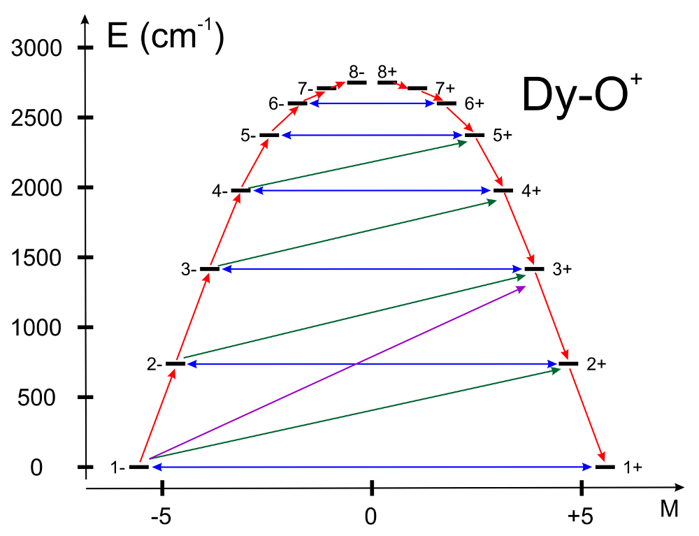
In this figure, a qualitative performance picture of the investigated single-molecular magnet is estimated by the strengths of the transition matrix elements of the magnetic moment connecting states with opposite magnetisaskytions (\(n+ \rightarrow n-\)). The height of the barrier is qualitatively estimated by the energy at which the matrix element (\(n+ \rightarrow n-\)) is large enough to induce significant tunnelling splitting at usual magnetic fields (internal) present in the magnetic crystals (0.01-0.1 Tesla). For the above example, the blocking barrier closes at the state (\(8+ \rightarrow 8-\)).
All transition matrix elements of the magnetic moment are given as \(((|\mu_X|+|\mu_Y|+|\mu_Z|)/3)\). The data is given in Bohr magnetons (\(\mu_{Bohr}\)).
Example:
UBAR true
ABCC_abcABCC_centerThe keywords
ABCC_abcandABCC_centerset the computation of magnetic and anisotropy axes in the crystallographic \(abc\) system. WithABCC_abc, the program reads six real values, namely \(a, b, c, \alpha, \beta\), and \(\gamma\), defining the crystal lattice. The values must be separated by a comma. WithABCC_center, the program reads the fractional coordinates of the magnetic center (from the CIF file) - again separated by comma. It is assumed that the XYZ coordinates used for the ab initio calculations did not rotate or translate the molecule from its crystallographic position. This input will ensure that all tensors computed bySINGLE_ANISOare given also in the \(abc\) system. The computed values in the output correspond to the crystallographic position of three “dummy atoms” located on the corresponding anisotropy axes, at the distance of 1.0 \(\mathring{A}\) from the metal site. Example:ABCC_abc 12.977, 12.977, 16.573, 90, 90, 120 ABCC_center 0.666667, 0.333333, 0.20413
XFIEThis keyword specifies the value (in T) of applied magnetic field for the computation of magnetic susceptibility by \(dM/dH\) and \(M/H\) formulas. A comparison with the usual formula (in the limit of zero applied field) is provided. (Default is 0.0). Example:
XFIE 0.35
This keyword together with the keyword
PLOTwill enable the generation of two additional plots:XT_with_field_dM_over_dH.pngandXT_with_field_M_over_H.png, one for each of the two above formula used, alongside with respectivegnuplotscripts and gnuplot datafiles.PLOTSet to “true”, the program generates a few plots (png or eps format) via an interface to the linux program gnuplot. The interface generates a datafile, a gnuplot script and attempts execution of the script for generation of the image. The plots are generated only if the respective function is invoked. The magnetic susceptibility, molar magnetisation and blocking barrier (
UBAR) plots are generated. The files are named:XT_no_field.dat,XT_no_field.plt,XT_no_field.png,MH.dat,MH.plt,MH.png,BARRIER_TME.dat,BARRIER_ENE.dat,BARRIER.pltandBARRIER.png,zeeman_energy_xxx.pngetc. All files produced bySINGLE_ANISOare referenced in the corresponding output section. Example:PLOT true
7.17.4. How to cite
We would appreciate if you cite the following papers in publications
resulting from the use of SINGLE_ANISO:
Chibotaru, L. F.; Ungur, L. J. Chem. Phys., 2012, 137, 064112.
Ungur, L. Chibotaru, L. F. Chem. Eur. J., 2017, 23, 3708-3718.
In addition, useful information like the definition of pseudospin Hamiltonians and their derivation can be found in this paper.