7.9. DeltaSCF: Converging to Arbitrary Single-Reference Wavefunctions
The regular SCF procedure is supposed to bring the wavefunction to a stationary point, and most times that means a minimum. However, sometimes one might want to converge to some kind of “excited state”, that is, a higher order saddle-point on the SCF surface.
Using the conventional SCF technology, it is usually not enough to start from an excited-state guess, but one needs to make some extra effort to keep the convergence towards that state. The stack of such methods to keep convergence to a given non-trivial state is called in the literature the DeltaSCF approach.
The general idea was first introduced by the group of Peter Gill [299] as the Maximum Overlap Method (MOM), and in ORCA we also feature the more recent PMOM from the group of Hrant Hratchian [184]. It has also been referred to as as “orbital optimized DFT for electronic excited states” [351].
To be very clear, let’s show one example in a picture:
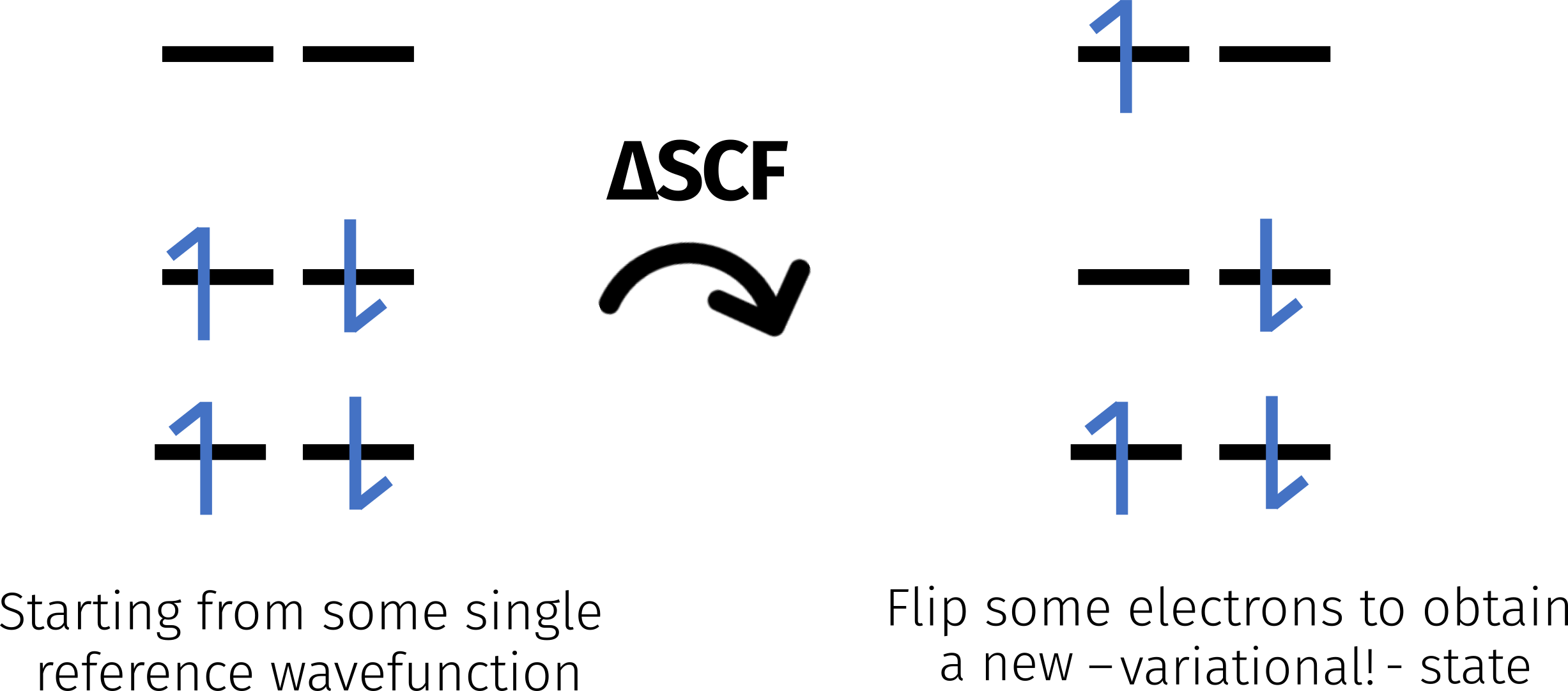
Fig. 7.2 A simple scheme of a HOMO-LUMO state using DeltaSCF
Using ORCA’s DeltaSCF, we can choose to converge the SCF to a HOMO/LUMO excited state. Now that excited state was obtained by fully relaxing the orbitals and can include any contributions such as the VV10 correlation or CPCM for solvation. We will also allow for gradients, geometry optimization, Hessian, EPR, NMR, or anything else that ORCA can do for a “normal” ground state calculation.
Important
The states obtained here are still represented by single-determinant wavefunctions, and in some cases might not even have physically correct meaning. Be careful and conscious of what you are doing! These are relatively reasonable wavefunctions for cases when:
the excited state can be simply described by a particle-hole interaction. That is for example NOT the case of a benzene molecule or most pi-pi* excited states.
the occupied and virtual orbitals are orthogonal or separated in space such that the relevant exchange integral is zero. Eg. some n-pi* states, orthogonal or long-distance charge separated states, etc;
for open-shell and doubly-excited states which can be represented by a single-determinant wavefunction.
7.9.1. First Example: HOMO-LUMO Excited State of Formaldehyde
Let’s begin by trying to converge and optimize to the first excited state of formaldehyde, starting from its regular planar structure:
!PBE DEF2-TZVP OPT FREQ DELTASCF UHF
%SCF ALPHACONF 0,1 END
* XYZ 0 1
C      0.000000    0.000000   -0.602985
O      0.000000    0.000000    0.605394
H      0.000000    0.934673   -1.182175
H      0.000000   -0.934673   -1.182175
*
Besides the regular keywords like method, basis set, OPT and FREQ, one needs to specify DELTASCF on the main input, and in this case, UHF, since the alpha and beta orbitals will be different (for doubly-excited states RHF is sufficient).
It is also necessary to add the ALPHACONF or BETACONF under the %SCF block. That is a minimal representation of the configuration you want to converge to. In this case, 0,1 means a HOMO/LUMO transition, where the HOMO has occupation zero and LUMO occupation one. For a HOMO-1/LUMO transition, it would be ALPHACONF 0,1,1. For a HOMO/LUMO+1 it would be ALPHACONF 0,0,1 and so on. Just picture how the frontier orbitals should look like. Any orbital below the first zero is assumed to be occupied and any orbital above the last occupied is assumed to be empty.
After the regular startup, the DeltaSCF-specific print shows:
-------------------------------
DELTA-SCF INITIAL CONFIGURATION
-------------------------------

Alpha: 1.00 1.00 1.00 0.00 1.00 0.00 0.00 0.00
Beta : 1.00 1.00 1.00 1.00 0.00 0.00 0.00 0.00

Hessian update                             ... L-SR1
Aufbau metric                              ... MOM
Keep initial reference                     ... true
Here you can follow the initial configuration and some other important things:
Hessian updaterefers to which method will be used for the SOSCF Hessian update. ORCA’s default isL-BFGS, which forces the electronic Hessian to be positive definite and will always push the system down to a minimum. As we want to go to a saddle point theL-SR1is set by default forDeltaSCF. More details on Hessian updates and their consequences at this reference from the group of Hannes Jónsson [510].Aufbau metricis the way one measures the “overlap” between the actual and reference wavefunctions (more details on [184]). It isMOMby default, but can be also set to%SCF PMOM TRUE ENDto usePMOM.Keep initial reference TRUEmeans we will always try to keep the initial reference state defined after the guess phase. That is sometimes calledIMOMin the literature [71]. If%SCF KEEPINITIALREF FALSE ENDis set, it is always the last SCF iteration that is taken as reference.
Important
Here are starting the orbitals from the PMODEL guess because it is trivial. In general we recommend always starting the SCF by reading the orbitals of a previously converged ground-state SCF! Please check Restarting SCF Calculations for more info on that.
This calculation trivially converges in 12 steps:
----------------------------------------D-I-I-S--------------------------------------------
Iteration    Energy (Eh)           Delta-E    RMSDP     MaxDP     DIISErr   Damp  Time(sec)
-------------------------------------------------------------------------------------------
               ***  Starting incremental Fock matrix formation  ***
MOM changed the orbital occupation numbers
    1    -114.2533654537761123     0.00e+00  2.06e-03  6.64e-02  7.14e-02  0.700   0.1
MOM changed the orbital occupation numbers
    2    -114.2675698961360382    -1.42e-02  4.71e-04  1.46e-02  3.08e-02  0.700   0.1
                               ***Turning on AO-DIIS***
MOM changed the orbital occupation numbers
    3    -114.2754325617175226    -7.86e-03  1.98e-04  3.98e-03  2.21e-02  0.700   0.1
MOM changed the orbital occupation numbers
    4    -114.2806616906060100    -5.23e-03  4.98e-04  6.40e-03  1.60e-02  0.000   0.1
MOM changed the orbital occupation numbers
                              *** Initializing SOSCF ***
---------------------------------------S-O-S-C-F--------------------------------------
Iteration    Energy (Eh)           Delta-E    RMSDP     MaxDP     MaxGrad    Time(sec)
--------------------------------------------------------------------------------------
    5    -114.2932665018211225    -1.26e-02  7.19e-05  1.55e-03  2.33e-03     0.1
               *** Restarting incremental Fock matrix formation ***
                            *** Restarting Hessian update ***
    6    -114.2932913947584979    -2.49e-05  5.82e-05  1.33e-03  1.11e-03     0.1
    7    -114.2932671856877818     2.42e-05  2.54e-05  5.00e-04  2.58e-03     0.1
    8    -114.2932914986330530    -2.43e-05  1.76e-05  3.20e-04  1.02e-03     0.1
    9    -114.2932961472105404    -4.65e-06  2.13e-06  6.94e-05  6.42e-05     0.1
   10    -114.2932961779292640    -3.07e-08  2.99e-05  1.10e-03  8.27e-06     0.1
   11    -114.2932921911087050     3.99e-06  3.05e-05  1.12e-03  5.44e-04     0.1
   12    -114.2932961794015654    -3.99e-06  2.45e-08  5.31e-07  2.39e-07     0.1
                  *** Gradient check signals convergence ***
Note
The statement MOM changed the orbital occupation numbers is normal, it is just printing what it is doing. Nothing to worry about.
and one can see from the spin contamination, that this is indeed an open-shell singlet:
----------------------
UHF SPIN CONTAMINATION
----------------------

Warning: in a DFT calculation there is little theoretical justification to
         calculate <S**2> as in Hartree-Fock theory. We will do it anyways
         but you should keep in mind that the values have only limited relevance

Expectation value of <S**2>     :     1.006910
Ideal value S*(S+1) for S=0.0   :     0.000000
Deviation                       :     1.006910
The gradient is then computed, and the geometry is optimized until convergence. Finally the frequencies show this is actually not a minimum, but a saddle point on the geometry space!
-----------------------
VIBRATIONAL FREQUENCIES
-----------------------

Scaling factor for frequencies =  1.000000000  (already applied!)

     0:       0.00 cm**-1
     1:       0.00 cm**-1
     2:       0.00 cm**-1
     3:       0.00 cm**-1
     4:       0.00 cm**-1
     5:       0.00 cm**-1
     6:    -591.31 cm**-1 ***imaginary mode***
     7:     799.56 cm**-1
     8:    1228.37 cm**-1
     9:    1271.29 cm**-1
    10:    2971.77 cm**-1
    11:    3067.96 cm**-1
The reason is: the HOMO/LUMO transition on formaldehyde populated the \(\pi^*\) LUMO, thus breaking the double bound and making the carbon atom pyramidal. If one starts from a slightly distorted structure, it then converges to the actual geometry minimum. Starting from a pyramidal structure:
!wB97M-D4 DEF2-TZVP DELTASCF UHF OPT FREQ
%SCF ALPHACONF 0,1 END
* XYZ 0 1
C          0.00000        0.00000       -0.60298
O         -0.74131       -0.10909        0.45746
H          0.00000        0.93467       -1.18217
H          0.00000       -0.93467       -1.18217
*
now converges to a minimum, as shown by the absence of negative frequencies:
-----------------------
VIBRATIONAL FREQUENCIES
-----------------------

Scaling factor for frequencies =  1.000000000  (already applied!)

     0:       0.00 cm**-1
     1:       0.00 cm**-1
     2:       0.00 cm**-1
     3:       0.00 cm**-1
     4:       0.00 cm**-1
     5:       0.00 cm**-1
     6:     713.25 cm**-1
     7:     826.75 cm**-1
     8:    1206.57 cm**-1
     9:    1292.70 cm**-1
    10:    2826.06 cm**-1
    11:    2893.16 cm**-1
The final geometry is surprisingly accurate for the gas phase formaldehyde too! We will also show the results here using the range-corrected, meta-GGA hybrid wB97M-D4 and the double-hybrid DFT !B2PLYP DEF2-QZVPP AUTOAUX, just to show that MP2 also works.
parameter |
exp. |
PBE |
wB97M-D4 |
B2PLYP |
|---|---|---|---|---|
r(C-O) |
1.323 |
1.300 |
1.310 |
1.311 |
r(C-H) |
1.098 |
1.113 |
1.093 |
1.090 |
\(\angle\)HCH |
118.8 |
115.0 |
117.0 |
116.8 |
\(\angle\)OOP |
34.0 |
41.1 |
36.5 |
37.0 |
exp. taken from [299].
Important
We are using the default SCF algorithm here, AO-DIIS + SOSCF because this is relatively simple. In general and for more complicated cases we suggest using directly the second order method, to avoid escaping back to the ground state with !NODIIS.
Important
Do NOT combine DeltaSCF wavefunctions with CCSD, or any such method with single excitations. It requires a speciallized version of CC which we don’t have yet.
Important
When running the same calculation above with wB97M-D4, there will not be a virtual orbital between the alpha HOMO-1 and the HOMO (so no negative HOMO-LUMO gap). There is nothing wrong here, it just optimized the orbitals to the excited state such that this is now a minimum on the SCF surface.
The energy is still higher than the non-DeltaSCF solution and if you plot the orbitals you will see that the alpha HOMO is now a \(\pi\) orbital instead of an \(n\).
7.9.2. Core-ionized States
Another big advantage of the DeltaSCF is the possibility to converge to core-excited and/or core-ionized states. We have a simple keyword to kick out electrons from any orbital, even the deep core ones:
%SCF IONIZEALPHA 2 END
and the electron from orbital number two will be removed. IONIZEBETA works for beta orbitals. One can start from an anion UHF -electronic structure obtained by adding one extra electron and remove a core electron like this to obtain core-excited states too. Geometry optimization, EPR, and even TD-DFT calculations are all valid for these states.
As an example, the input below will ionize the 1s electron from a water molecule, which corresponds to MO 0 here:
!PBE0 DEF2-TZVP DELTASCF NODIIS UHF
%SCF IONIZEALPHA 0 END
* xyz 0 1
  O      2.127880   -0.361920    0.104770
  H      3.117210   -0.387460    0.070360
  H      1.838520   -0.926280   -0.655730
*
Note
If the orbital is not localized over a single atom one might need to localized them first!
and one can see from the results that is exactly where it converged to.
----------------
ORBITAL ENERGIES
----------------
                 SPIN UP ORBITALS
  NO   OCC          E(Eh)            E(eV)
   0   0.0000     -20.108086      -547.1688
   1   1.0000      -1.567415       -42.6515
   2   1.0000      -1.057257       -28.7694
   3   1.0000      -0.939315       -25.5601
   4   1.0000      -0.882871       -24.0241
   5   0.0000      -0.304254        -8.2792
   6   0.0000      -0.239285        -6.5113
   7   0.0000       0.044344         1.2066
        (...)
Note
ORCA automatically adjusts charge and multiplicity here. The input should contain those from the reference system!
Here are some examples of binding energies for 1s electrons. The atom from where it was removed is highlighted in bold:
1s ionization |
exp. |
wB97M-V |
|---|---|---|
H2O |
539.82 |
541.17 |
CO2 |
297.69 |
299.10 |
NH3 |
405.56 |
406.82 |
CH3CN |
405.64 |
406.92 |
exp. taken from [143]
7.9.3. Diabatic Couplings
DeltaSCF is also a quite accurate method to obtained diabatic couplings, which can later be used in Markus theory to compute electron transfer rates. These can be computed by calculating the energy difference between electron transfer states and using the Generalized Mulliken-Hush Approach (GMH). For more details please check for example this paper from the group of Blumberger [477].
There is not enough space to go through the details here, but one can get these diabatic coupling from essentially one regular SCF for the ground state + a DeltaSCF for the excited state. For symmetric systems, this is trivial:
where states \(a\) and \(b\) are diabatic states \(\Delta E_{12}\) is the energy difference between adiabatic states \(1\) and \(2\) (which are obtained via SCF solution). Here is an example of the diabatic couplings obtained for a benzene dimer, obtained by starting from the ground state cation and exciting the beta electron with:
%SCF BETACONF 0,1 END
Distance in Ang |
MRCI+Q |
wB97M-V |
TD-DFT |
|---|---|---|---|
3.5 |
435.2 |
473.1 |
593 |
4.0 |
214.3 |
236.7 |
374 |
4.5 |
104.0 |
115.9 |
267.5 |
5.0 |
51.70 |
56.7 |
218.5 |
MRCI+Q taken from [477]
Note
There is more to come with respect to DeltaSCF. We are collaborating further with Prof. Hannes Jónsson’s group - stay tuned.
7.9.4. Full keyword list
Here we present a complete list of options to be given under %SCF related to DeltaSCF:
%SCF

   #
   # general options
   #

   DOMOM          TRUE  # do the reordering of the orbitals at all? (default TRUE)
   KEEPINITIALREF TRUE  # always keep initial reference: IMOM? (default TRUE)

   PMOM           FALSE # use the PMOM metric instead of the regular MOM? (default FALSE)

   #
   # occupation number
   #

   ALPHACONF      0,1    # define the occupation of the frontier orbitals.
                         # for RHF and doubly occupied states it could be 0,2.
   BETACONF       0,0,1  # same for the beta orbitals.

   IONIZEALPHA    23     # remove electron from alfa MO number 23?
   IONIZEBETA     12     # remove electron from alfa MO number 12?

   #
   # SOSCF Hessian update
   #

   SOSCFHESSUP    LSR1     # symmetryc rank-1 update (default and recommended).
                  LBFGS    # L-BFGS update.
                  LPOWELL  # regular L-Powell update.
                  LBOFILL  # Bofill update, a combination of SR1 and Powell.