6.18. Excited State Dynamics
ORCA can now also be used to compute dynamic properties involving excited
states such as absorption spectra, fluorescence and phosphorescence rates
and spectra, as well as resonant Raman spectra using the new ORCA_ESD
module. We do this by analytically solving the Fermi’s Golden Rule-like
equation from Quantum Electrodynamics (see the section More on the Excited State Dynamics module),
using a path integral approach to the dynamics, as described in our recent papers
[198, 199]. The computation of these rates
relies on the harmonic approximation for the nuclear normal modes. Provided
this approximation holds, the results closely match experimental data.
The theory can do most of what ORCA_ASA can and more, such as including
vibronic coupling in forbidden transitions (the so-called Herzberg-Teller
effect, HT), considering Duschinsky rotations between modes of different
states, solving the equations using different coordinate systems, etc.
There are also seven new approaches to obtain the excited state geometry
and Hessian without necessarily optimizing its geometry. Many keywords
and options are available, but most of the defaults already give good results.
Let’s get into specific examples, starting with the absorption spectrum.
Please refer to section More on the Excited State Dynamics module for a complete keyword list and details.
6.18.1. Absorption Spectrum
6.18.1.1. The ideal model, Adiabatic Hessian (AH)
To predict absorption or emission rates, including all vibronic transitions, ideally, one requires both the ground state (GS) and excited state (ES) geometries and Hessians. For instance, when predicting the absorption spectrum for benzene, which exhibits one band above 220 nm corresponding to a symmetry-forbidden excitation to the S1 state, the process is straightforward. Ground state information can be obtained from (Sec. Geometry Optimizations, Surface Scans, Transition States, MECPs, Conical Intersections, IRC, NEB):
!B3LYP DEF2-SVP OPT FREQ
* XYZFILE 0 1 BEN.xyz
and the S1 ES from (Sec. Excited State Geometry Optimization):
!B3LYP DEF2-SVP OPT FREQ
%TDDFT
  NROOTS   5
  IROOT    1
END
* XYZFILE 0 1 BEN_S1.xyz
Assuming DFT/TD-DFT here, but other methods can also be used (see Tips, Tricks and Troubleshooting). With both Hessians available, the ESD module can be accessed from:
!B3LYP DEF2-SVP TIGHTSCF ESD(ABS)
%TDDFT
  NROOTS     5
  IROOT      1
END
%ESD
  GSHESSIAN  "BEN.hess"
  ESHESSIAN  "BEN_S1.hess"
  DOHT       TRUE
END
* XYZFILE 0 1 BEN.xyz
Important
The geometry must match that in the GS Hessian when calling the ESD module. You can obtain it from the .xyz file after geometry optimization or directly copy it from the .hess file (remember to use BOHRS on the input to correct the units, if obtained from the .hess).
You must provide both names for the Hessians and set DOHT to TRUE here because the first transition of benzene is symmetry forbidden, with an oscillator strength of 2e-6. Therefore, all intensity arises from vibronic coupling (HT effect) [199]. In molecules with strongly allowed transitions, this parameter can typically remain FALSE (the default). Some calculation details are printed, including the computation of transition dipole derivatives for the HT component, and the spectrum is saved as BASENAME.spectrum.
Energy                  TotalSpectrum           IntensityFC             IntensityHT
10807.078728            2.545915e-02            2.067393e-07            2.545894e-02
10828.022679            2.550974e-02            2.071508e-07            2.550954e-02
10848.966630            2.556034e-02            2.075624e-07            2.556013e-02
...
The first column has the total spectrum, but the contributions from the Franck-Condon part and the Herzberg-Teller part are also discriminated. As you can see, the FC intensity is less than 1% of the HT intensity here, highlighting the importance of including the HT effect. It is important to note that, in theory, the absorbance intensity values correspond to the experimental \(\varepsilon\) (in L mol cm\(^{-1}\)), and they depend on the spectral lineshape. The TotalSpectrum column can be plotted using any software to obtain the spectrum named Full AH spectrum (shown in blue), in Fig. 6.58 below.

Fig. 6.58 Here is the experimental absorption spectrum for benzene (shown in black on the left), alongside predictions made using ORCA_ESD at various PES approximations.
The spectrum obtained is very close to the experimental results at 298K, even when simply using all the defaults, and it could be further improved by adjusting parameters such as lineshape, as discussed in detail in Sec. General Aspects and Sec. More on the Excited State Dynamics module.
Note
The path integral approach in ORCA_ESD is much faster than the more traditional approach of calculating all vibronic transitions with non-negligible intensities, one by one [748]. This is especially true for large systems, where the number of bright vibronic transitions may potentially scale exponentially, but our approach’s scaling remains polynomial (in fact near linear scaling in favorable cases [199]). The price to pay is that one can no longer read off the compositions of the vibronic states from the spectrum, in other words, one cannot assign the peaks without doing further calculations. However, one can know whether a given vibrational mode contributes to a given peak, by repeating the ESD calculation with a few modes removed, and see if the peak is still present. This can be conveniently done using the MODELIST or SINGLEMODE keywords. More information can be found in Sec. More on the Excited State Dynamics module.
The Huang-Rhys factors are important tools for qualitative and quantitative analysis of the contributions of each vibrational mode to the vibrationally resolved spectrum (and also to the transition rate constants, as will be discussed later). They can be requested by setting PRINTLEVEL in the %ESD module to 3 or above.
Of course, it is not always possible to obtain the excited state (ES) geometry due to root flipping, or it might be too costly for larger systems. Therefore, some approximations to the ES Potential Energy Surface (PES) have been developed.
6.18.1.2. The simplest model, Vertical Gradient (VG)
The minimal approximation, known as Vertical Gradient (VG), assumes that the excited state (ES) Hessian equals the ground state (GS) Hessian and extrapolates the ES geometry from the ES gradient and that Hessian using some step (Quasi-Newton or Augmented Hessian, which is the default here). Additionally, in this scenario, the simplest Displaced Oscillator (DO) model is employed, ensuring fast computation [199]. To use this level of approximation, simply provide an input like:
!B3LYP DEF2-SVP TIGHTSCF ESD(ABS)
%TDDFT
  NROOTS     5
  IROOT      1
END
%ESD
  GSHESSIAN  "BEN.hess"
  DOHT       TRUE
  HESSFLAG   VG    #DEFAULT
END
* XYZFILE 0 1 BEN.xyz
OBS: If no GSHESSIAN is given, it will automatically look for an BASENAME.hess file.
Choosing one of the methods in ORCA to compute excited state information is essential. Here, we utilize TD(A)-DFT with IROOT 1 to compute properties for the first excited state. TD(A)-DFT is currently the sole method offering analytic gradients for excited states; selecting any other method will automatically enforce NUMGRAD.
Important
Please note that certain methods, such as STEOM-DLPNO-CCSD, require significant time to compute numerical gradients. In such cases, we recommend using DFT/TD-DFT Hessians and employing the higher-level method solely for single points.
If everything is set correctly, after the regular single point calculation, the ESD module in ORCA will initiate. It proceeds to obtain the excited state (ES) geometry, compute derivatives, and predict the spectrum. The resulting normalized spectrum can be observed in Fig. 6.58, depicted in red. Due to such simple model, the spectrum is also simplified. While this simplicity is less critical for larger molecules, it highlight the potential benefit of employing an intermediate model.
6.18.1.3. A better model, Adiabatic Hessian After a Step (AHAS)
A reasonable compromise between a full geometry optimization and a simple step with the same Hessian is to perform a step and then recalculate the ES Hessian at that geometry. This approach is referred to here as Adiabatic Hessian After Step (AHAS). In our tests, it can be invoked with the following input:
!B3LYP DEF2-SVP TIGHTSCF ESD(ABS)
%TDDFT
  NROOTS     5
  IROOT      1
END
%ESD
  GSHESSIAN  "BEN.hess"
  DOHT       TRUE
  HESSFLAG   AHAS
END
* XYZFILE 0 1 BEN.xyz
The spectrum obtained corresponds to the green line in Fig. 6.58. As shown, it closely resembles the spectrum obtained using AH, where a full geometry optimization was performed. Although not set as the default, this method comes highly recommended based on our experience [199]. Another advantage of this approach is that the derivatives of the transition dipole are computed simultaneously over Cartesian displacements on the ES structure using the numerical Hessian. Subsequently, these modes are straightforwardly converted.
OBS: The transition dipoles used in our formulation are always those of the FINAL state geometry. For absorption, this corresponds to the ES, so in AHAS, the derivatives are computed over this geometry. For fluorescence, the default behavior is to recompute the derivatives over the GS geometry. Alternatively, you can choose to save time and convert directly from ES to GS by setting CONVDER TRUE (though this is an approximation). For more details, refer to Sec. More on the Excited State Dynamics module.
6.18.1.4. Other PES options
There are also a few other options that can be set using HESSFLAG. For example, you can calculate the vertical ES Hessian over the GS geometry and perform a step, known as the Vertical Hessian (HESSFLAG VH) method. This method has the advantage that the geometry step is expected to be better because it does not assume the initial ES Hessian is equal to the GS Hessian. However, it is likely to encounter negative frequencies on that VH, since you are not at the ES minimum. By default, ORCA will turn negative frequencies into positive ones, issuing a warning if any were lower than -300 cm\(^{-1}\). You can also choose to completely remove them (and the corresponding frequencies from the GS) by setting IFREQFLAG to REMOVE or leave them as negative with IFREQFLAG set to LEAVE under %ESD. Just be aware that an odd number of negative frequencies might disrupt the calculation of the correlation function, so be sure to check.
If your excited state is localized and you prefer not to recalculate the entire Hessian, you can opt for a Hybrid Hessian (HH) approach. This involves recomputing the ES Hessian only for specific atoms listed in HYBRID_HESS under %FREQ (Frequency calculations - numerical and analytical). The HH method uses the GS Hessian as a base but adjusts it at the specified atoms. This computation can be performed either before or after the step, offering two variations: Hybrid Hessian Before Step (HESSFLAG HHBS) or Hybrid Hessian After Step (HESSFLAG HHAS). When using either of these options, derivatives are recalculated across the modes as needed.
Another approach involves comparing the ES Hessian with the GS Hessian and selectively recomputing frequencies that differs. This method works by applying a displacement based on the GS Hessian and evaluating the resulting energy change. If the predicted mode matches the actual mode, the prediction should be accurate. However, if the difference exceeds a specified threshold, the gradient is computed, and the frequency for that mode is recalculated accordingly. The final ES Hessian is then derived from the Updated Frequencies (UF) and the original GS Hessian.
This approach offers the advantage of minimizing the computation of ES gradients typical in standard ES Hessians, thereby speeding up the process. By default, the system checks for frequency errors of approximately 20%. You can adjust this threshold using the UPDATEFREQERR flag; for instance, setting UPDATEFREQERR to 0.5 under %ESD allows for a larger error tolerance of 50%. Additionally, you can implement either the Updated Frequencies Before Step (HESSFLAG UFBS) or the Updated Frequencies After Step (UFAS) methods. Transition dipole derivatives are computed concurrently with the update process.
OBS: All these options apply to Fluorescence and resonant Raman as well.
6.18.1.5. Duschinsky rotations
The ES modes can sometimes be expressed as linear combinations of the GS modes (see Sec. General Aspects of the Theory), a phenomenon known in the literature as Duschinsky rotation [228]. In our formulation within ORCA_ESD, it is possible to account for this effect, which reflects a closer approximation to real-world scenarios, albeit at a higher computational cost.
You can enable this feature by setting USEJ TRUE; otherwise, the rotation matrix J defaults to unity. For instance, in the case of benzene, while the effect may not be pronounced, there is noticeable improvement in matching peak ratios with experimental data when incorporating rotations. Exploring this option may reveal more significant impacts in other cases.

Fig. 6.59 Experimental absorption spectrum for benzene (black on the left) and the effect of Duschinsky rotation on the spectrum.
6.18.1.6. Temperature effects
In our model, the effects of the Boltzmann distribution due to temperature are exactly accounted for [199]. The default temperature is set to 298.15 K, but you can specify any other temperature by adjusting the TEMP parameter under %ESD. However, it is important to note that when approaching temperatures close to 0 K, numerical issues may arise. For instance, if you encounter difficulties modeling a spectrum at 5 K or wish to predict a jet-cooled spectrum, setting TEMP to 0 will activate a set of equations specifically tailored for T=0 K conditions.
As can be seen in Fig. 6.60, at 0 K there are no hot bands and fewer peaks, while at 600 K there are many more possible transitions due to the population distribution over the GS.

Fig. 6.60 Predicted absorption spectrum for benzene at different temperatures.
6.18.1.7. Multistate Spectrum
If you want to predict a spectrum that includes many different states, you should ignore the IROOT flag in all modules and instead use the STATES flag under %ESD. For example, to predict the absorption spectra of pyrene in the gas phase and consider the first twenty states, you would specify:
!B3LYP DEF2-TZVP(-F) TIGHTSCF ESD(ABS)
%TDDFT
  NROOTS     20
END
%ESD
  GSHESSIAN  "PYR.hess"
  ESHESSIAN  "PYR_S1.hess"
  DOHT       TRUE
  STATES     1,2,3,4,5,6,7,8,9,10,11,12,13,14,15,16,17,18,19,20
  UNIT       NM
END
* XYZFILE 0 1 PYR.xyz
This input would result in the spectra shown in Fig. 6.61. In this case, each individual spectrum for every state will be saved as BASENAME.spectrum.root1, BASENAME.spectrum.root2, etc., while the combined spectrum, which is the sum of all individual spectra, will be saved as BASENAME.spectrum.

Fig. 6.61 Predicted absorption spectrum for pyrene in gas phase (solid blue) in comparison to the experiment (dashed grey) at 298 K.
OBS: The flag UNIT can be used to control the output unit of the X axis. Its values can be CM-1, NM or EV and it only affects the OUTPUT, the INPUT should always be in cm\(^{-1}\)
6.18.2. Fluorescence Rates and Spectrum
6.18.2.1. General Aspects
The prediction of fluorescence rates and spectra can be performed in a manner analogous to absorption, as described above, by using ESD(FLUOR) on the main input line. You can select any of the methods described earlier to obtain the Potential Energy Surface (PES) by setting the appropriate HESSFLAG. The primary distinction is that the transition dipoles must correspond to the geometry of the ground state (GS), while all other aspects remain largely unchanged.

Fig. 6.62 Predicted absorption (right) and emission (left) spectrum for benzene in hexane at 298.15 K.
As depicted in Fig. 6.62, the fluorescence spectrum also closely matches the experimental data [199]. The difference observed in the absorption spectrum in Fig. 6.62, compared to previous spectra, arises because the experiment was conducted in a solvent environment. Therefore, we adjusted the linewidth to align with the experimental data.
OBS: It is common for the experimental lineshape to vary depending on the setup, and this can be adjusted using the LINEW flag (in cm\(^{-1}\)). There are four options for the lineshape function controlled by the LINES flag: DELTA (for a Dirac delta function), LORENTZ (default), GAUSS (for a Gaussian function), and VOIGT (a Voigt profile, which is a product of Gaussian and Lorentzian functions).
OBS2: The DELE and TDIP keywords can be used to input adiabatic (not vertical!) excitation energy and transition dipole moment computed at a higher level of theory. This enables calculating the computationally intensive Hessians (especially the excited state Hessian) at a low level of theory without compromising the accuracy. For more details, see Sec. Mixing methods.
If you need to control the lineshapes separately for Gaussian (GAUSS) and Lorentzian (LORENTZ), you can set LINEW for Lorentzian and INLINEW for Gaussian (where “I” stands for Inhomogeneous Line Width).
!B3LYP DEF2-SVP TIGHTSCF ESD(FLUOR)
%TDDFT
  NROOTS     5
  IROOT      1
END
%ESD
  GSHESSIAN  "BEN.hess"
  ESHESSIAN  "BEN_S1.hess"
  DOHT       TRUE
  LINES      VOIGT
  LINEW      75
  INLINEW    200
END
* XYZFILE 0 1 BEN.xyz
OBS: The LINEW and INLINEW are NOT the full width half maximum (\(FWHM\)) of these curves. However, they are related to them by: \(FWHM_{lorentz} = 2 \times LINEW\); \(FWHM_{gauss} = 2.355 \times INLINEW\).
For the VOIGT curve, it is a little more complicated but in terms of the other FWHMs, it can be approximated as: \(FWHM_{voigt} = 0.5346 \times FWHM_{lorentz} + \sqrt{(0.2166 \times FWHM_{lorentz}^2 + FWHM_{gauss}^2) }\).
6.18.2.2. Rates and Examples
When you select ESD(FLUOR) on the main input, the fluorescence rate will be printed at the end of the output, with contributions from Franck-Condon (FC) and Herzberg-Teller (HT) mechanisms discriminated. If you use CPCM, the rate will be multiplied by the square of the refractive index, following Strickler and Berg [831].
If you calculate a rate without CPCM but still want to account for the solvent effect, remember to multiply the final rate by this factor. Below is an excerpt from the output of a calculation with CPCM (hexane):
Warning
Whenever using ESD with CIS/TD-DFT and solvation, CPCMEQ will be set to TRUE by default, since the excited state should be under equilibrium conditions! More info in Including solvation effects via LR-CPCM theory.
...
          ***Everything is set, now computing the correlation function***

Homogeneous linewidht is:			50.00 cm-1
Number of points:				131072
Maximum time:					1592.65 fs
Spectral resolution:				3.33 cm-1
Temperature used:				298.15 K
Z value:					5.099843e-42
Energy difference:				41049.37 cm-1
Reference transition dipole (x,y,z):		(0.00004 0.00000),
                                    		(0.00002 0.00000),
                                    		(-0.00058 0.00000)
Calculating correlation function:		...done
Last element of the correlation function:	0.000000,-0.000000
Computing the Fourier Transform:		...done

The calculated fluorescence rate constant is	1.688355e+06 s-1*
with 0.00% from FC and 100.00% from HT

*The rate is multiplied by the square of the refractive index

The fluorescence spectrum was saved in		BASENAME.spectrum
In one of our theory papers, we investigated the calculation of fluorescence rates for the set of molecules presented in Fig. 6.63. The results are summarized in Fig. 6.64 for some of the methods used to obtain the Potential Energy Surface (PES) mentioned.

Fig. 6.63 The set of molecules studied, with rates on Fig. 6.64.

Fig. 6.64 Predicted emission rates for various molecules in hexane at 298.15 K. The numbers below the labels are the HT contribution to the rates.
6.18.3. Phosphorescence Rates and Spectrum
6.18.3.1. General Aspects
As with fluorescence, phosphorescence rates and spectra can be calculated if spin-orbit coupling is included in the excited state module (please refer to the relevant publication [198]). To enable this, ESD(PHOSP) must be selected in the main input, and both a GSHESSIAN and a TSHESSIAN must be provided. The triplet Hessian can be computed analytically from the spin-adapted triplets.
!B3LYP DEF2-TZVP(-F) CPCM(ETHANOL) OPT FREQ
%TDDFT
  NROOTS 5
  IROOTMULT TRIPLET
END
* XYZ 0 1
C         -0.82240       -0.05739        0.00515
C          0.42295        0.77803        0.02146
H         -0.85252       -0.69527        0.89195
H         -0.85090       -0.66429       -0.90325
H         -1.69889        0.59680        0.01431
C          1.74379        0.02561       -0.01818
C          2.98907        0.86121       -0.00686
H          3.01366        1.50199       -0.89176
H          3.86561        0.20724       -0.02398
H          3.02300        1.46514        0.90332
O          0.42398        2.00161        0.06749
O          1.74282       -1.19814       -0.05965
*
or, in this case, by computing the ground state triplet by simply setting the multiplicity to three:
!B3LYP DEF2-TZVP(-F) CPCM(ETHANOL) OPT FREQ
* XYZFILE 0 3 BIA.xyz
Alternatively, one can use methods like VG, AHAS, etc., to approximate the triplet geometry and Hessian. However, this approach requires preparing the Hessian in a separate ESD run (Sec. Approximations to the excited state PES).
Additionally, you must input the adiabatic energy difference between the ground singlet and ground triplet states at their respective geometries (without any zero-point energy correction) using the DELE flag under %ESD. In this case, the spin-adapted triplet computed previously serves as our reference triplet state. An example input for the rate calculation using TDDFT is as follows:
!B3LYP DEF2-TZVP(-F) TIGHTSCF CPCM(ETHANOL) ESD(PHOSP) RI-SOMF(1X)
%TDDFT
  NROOTS  20
  DOSOC   TRUE
  TDA     FALSE
  IROOT   1
END
%ESD    GSHESSIAN       "BIA.hess"
        TSHESSIAN       "BIA_T1.hess"
        DOHT            TRUE
        DELE            17260
END
* XYZFILE 0 1 BIA.xyz

$NEW_JOB

!B3LYP DEF2-TZVP(-F) TIGHTSCF CPCM(ETHANOL) ESD(PHOSP) RI-SOMF(1X)
%TDDFT
  NROOTS  20
  DOSOC   TRUE
  TDA     FALSE
  IROOT   2
END
%ESD    GSHESSIAN       "BIA.hess"
        TSHESSIAN       "BIA_T1.hess"
        DOHT            TRUE
        DELE            17260
END
* XYZFILE 0 1 BIA.xyz

$NEW_JOB

!B3LYP DEF2-TZVP(-F) TIGHTSCF CPCM(ETHANOL) ESD(PHOSP) RI-SOMF(1X)
%TDDFT
  NROOTS  20
  DOSOC   TRUE
  TDA     FALSE
  IROOT   3
END
%ESD    GSHESSIAN       "BIA.hess"
        TSHESSIAN       "BIA_T1.hess"
        DOHT            TRUE
        DELE            17260
END
* XYZFILE 0 1 BIA.xyz
Phosphorescence rate calculation are always accompanied by the generation of the vibrationally resolved phosphorescence spectrum, which can be visualized in the same way as fluorescence spectra.
OBS.: When computing phosphorescence rates, each rate from individual
spin sub-levels must be requested separately. You may use the $NEW_JOB
option, just changing the IROOT, to write everything in a single input.
After SOC, the three triplet states (\(T_1\) with \(M_S\) = -1, 0 and +1) will
split into IROOTs 1, 2 and 3, and all of them must be included when
computing the final phosphorescence rate. In this case, it is reasonable
to assume that the geometries and Hessians of these spin sub-levels are
the same, and we will use the same .hess file for all three.
OBS2.: The ground state geometry should be used in the input file, similar to the case of fluorescence (vide supra).
OBS3.: Apart from DELE, one can also use the TDIP keyword to input a high-level transition dipole moment, similar to the fluorescence case. This enables e.g. the calculation of phosphorescence rates/spectra using e.g. NEVPT2 or DLPNO-STEOM-CCSD transition dipole moments, with (TD)DFT geometries and Hessians. Note however that the transition dipole moment in phosphorescence processes is complex, so 6 instead of 3 components are required.
Here, we are computing the rate and spectrum for biacetyl in ethanol at 298 K. The geometries and Hessians were obtained as previously described, with the ground triplet computed from a simple open-shell calculation. To compute the rate, the flag DOSOC must be set to TRUE under %TDDFT (Sec Spin-orbit coupling), or the respective module, and it is advisable to set a large number of roots to ensure a good mixing of states.
Please note that we have chosen the RI-SOMF(1X) option for the spin-orbit coupling integrals, but any of the available methods can be used (Sec. The Spin-Orbit Coupling Operator).
6.18.3.2. Calculation of rates
As you can see, the predicted spectra for biacetyl (Fig. 6.65) are quite close to the experimental results [198, 784]. The calculation of the phosphorescence rate is more complex because there are three triplet states that contribute. Therefore, the observed rate must be taken as an average of these three states.
To be even more strict and account for the Boltzmann population distribution at a given temperature \(T\) caused by the Zero Field Splitting (ZFS), one should use [593]:
where \(\Delta E_{1,2}\) is the energy difference between the first and second states, and so on.
After completion of each calculation, the rates for the three triplets were 8.91 s\(^{-1}\), 0.55 s\(^{-1}\), and 284 s\(^{-1}\). Using (6.26), the final calculated rate is about 98 s\(^{-1}\), while the best experimental value is 102 s\(^{-1}\) (at 77K) [592], with about 40% deriving from the HT effect.

Fig. 6.65 The experimental (dashed red) and theoretical (solid black, displaced by about 2800 cm\(^{-1}\)) phosphorescence spectra for biacetyl, in ethanol at 298 K.
OBS: A subtlety arises when the final state is not a singlet state, for example in radical phosphorescence (doublet ground state) or singlet oxygen phosphorescence (triplet ground state). In this case the most rigorous treatment would be to sum over the final states but average over the initial states. For example, with quartet-to-doublet phosphorescence one gets
where \(k_{2\to 1}\) is the phosphorescence rate constant from the second sublevel of the initial quartet to the first sublevel of the final doublet, etc. Note that the Boltzmann factors of the final state do not enter the expression. Unfortunately, since U-TDDFT is spin contaminated and unsuitable for calculating SOC-corrected transition dipole moments, the transition dipoles in this case have to be calculated by more advanced methods, such as DFT/ROCIS or multireference methods. The transition dipole should then be given in the input file using the TDIP keyword.
6.18.4. Intersystem Crossing Rates (unpublished)
6.18.4.1. General Aspects
Yet another application of the path integral approach is to compute intersystem crossing rates, or non-radiative transition rates between states of different multiplicities. This can be calculated if one has two geometries, two Hessians, and the relevant spin-orbit coupling matrix elements.
The input is similar to those discussed above. Here ESD(ISC) should be used on the main input to indicate an InterSystem Crossing calculation, and the Hessians should be provided by ISCISHESSIAN and ISCFSHESSIAN for the initial and final states, respectively. Please note that the geometry used in the input file should correspond to that of the FINAL state, specified through the ISCFSHESSIAN flag. The relevant matrix elements can be computed using any method available in ORCA and inputted as SOCME Re,Im under %ESD where Re and Im represent its real and imaginary parts (in atomic units!).
As a simple example, one could compute the excited singlet and ground triplet geometries and Hessians for anthracene using TD-DFT. Then, compute the spin-orbit coupling (SOC) matrix elements for a specific triplet spin-sublevel using the same method (see the details below), potentially employing methods like CASSCF, MRCI, STEOM-CCSD, or another theoretical level. Finally, obtain the intersystem crossing (ISC) rates using an input such as:
!ESD(ISC) NOITER
%ESD
  ISCISHESSIAN  "ANT_S1.hess"
  ISCFSHESSIAN  "ANT_T1.hess"
  DELE          11548
  SOCME         0.0, 2.33e-5
END
* XYZFILE 0 1 ANT_T1.xyz
The SOCMEs between a singlet state and a triplet state consist of three complex numbers, not just one, because the triplet state has three sublevels. If the user uses the SOCME of one of the sublevels as input to the ISC rate calculation, this gives the ISC rate associated with that particular sublevel. However, experimentally one usually does not distinguish the three sublevels of a triplet state, and experimentally ISC rates are reported as if the three sublevels of a triplet state are the same species. Therefore, the rate of singlet-to-triplet ISC is the sum of the ISC rates from the singlet state to the three triplet sublevels. Fortunately, in case the Herzberg-Teller effect (vide infra) can be neglected, it is not necessary to perform three rate calculations and add up the rates, since the rate is proportional to the squared modulus of the SOCME. Thus, one can run a single ESD calculation where the SOCME is the square root of the summed squared moduli of the three SOCME components.
As an illustration, consider the \(S_1\) to \(T_1\) ISC rate of acetophenone. First, we optimize the \(S_0\) geometry, and (after manually tweaking the geometry to break mirror symmetry) use it as an initial guess for the geometry optimization and frequency calculations of the \(S_1\) and \(T_1\) states. Then, we calculate the \(S_1\)-\(T_1\) SOCMEs at the \(T_1\) geometry (note that, as usual, final state geometries should be used for ESD calculations; this may differ from some programs other than ORCA). These calculations are conveniently done using a compound script, although the individual steps can of course also be done using separate input files.
%pal nprocs 16 end

* xyz 0 1
  C      1.512698    7.783764   -0.013405
  C      2.900029    7.735359   -0.016012
  C      3.664170    8.950745    0.000408
  C      2.952045   10.199539    0.007630
  C      1.564497   10.214795    0.009890
  C      0.827311    9.015246    0.000726
  H      0.946857    6.847253   -0.027731
  H      3.394565    6.763402   -0.041976
  H      3.505090   11.140193    0.017889
  H      1.039592   11.175094    0.019479
  H     -0.265468    9.038211    0.000969
  C      5.059695    8.958412    0.000442
  O      5.733735   10.161120   -0.048672
  C      5.927824    7.713913    0.020029
  H      5.442615    6.938582    0.639989
  H      6.073177    7.326421   -1.014490
  H      6.923426    7.950459    0.447785
 *

%compound

new_step # Compound 1: S1 opt
! B3LYP def2-SV(P) opt tightopt freq

%tddft
tda false
nroots 2
iroot 1
end

step_end

new_step # Compound 2: T1 opt
! B3LYP def2-SV(P) opt tightopt freq

* xyz 0 3
  C      1.512698    7.783764   -0.013405
  C      2.900029    7.735359   -0.016012
  C      3.664170    8.950745    0.000408
  C      2.952045   10.199539    0.007630
  C      1.564497   10.214795    0.009890
  C      0.827311    9.015246    0.000726
  H      0.946857    6.847253   -0.027731
  H      3.394565    6.763402   -0.041976
  H      3.505090   11.140193    0.017889
  H      1.039592   11.175094    0.019479
  H     -0.265468    9.038211    0.000969
  C      5.059695    8.958412    0.000442
  O      5.733735   10.161120   -0.048672
  C      5.927824    7.713913    0.020029
  H      5.442615    6.938582    0.639989
  H      6.073177    7.326421   -1.014490
  H      6.923426    7.950459    0.447785
 *

step_end

new_step # Compound 3: SOC at T1 geometry
! B3LYP def2-SV(P)

%tddft
tda false
nroots 3
triplets true
dosoc true
end

# Here it is assumed that the input file is named "a.inp"
* xyzfile 0 1 a_Compound_2.xyz

step_end
end
After verifying that neither of the Hessians have imaginary frequencies (which is very important!), we can read the computed SOCMEs:
      --------------------------------------------------------------------------------
                      CALCULATED SOCME BETWEEN TRIPLETS AND SINGLETS
      --------------------------------------------------------------------------------
           Root                          <T|HSO|S>  (Re, Im) cm-1
         T      S             Z                     X                     Y
      --------------------------------------------------------------------------------
         1      0    (   0.00 ,   -2.00 )    (   0.00 ,   29.24 )    (  -0.00 ,  -41.11 )
         1      1    (   0.00 ,   -0.59 )    (   0.00 ,    1.79 )    (  -0.00 ,   -2.57 )
         1      2    (   0.00 ,    0.52 )    (   0.00 ,   -3.19 )    (  -0.00 ,    3.21 )
         1      3    (   0.00 ,   -2.39 )    (   0.00 ,   14.57 )    (  -0.00 ,  -19.53 )
         2      0    (   0.00 ,   -0.11 )    (   0.00 ,    2.78 )    (  -0.00 ,   -2.72 )
         2      1    (   0.00 ,    2.25 )    (   0.00 ,  -20.07 )    (  -0.00 ,   28.07 )
         2      2    (   0.00 ,    0.02 )    (   0.00 ,   -0.13 )    (  -0.00 ,    0.29 )
         2      3    (   0.00 ,   -0.17 )    (   0.00 ,    0.59 )    (  -0.00 ,   -1.27 )
         3      0    (   0.00 ,   -0.01 )    (   0.00 ,    0.05 )    (  -0.00 ,   -0.06 )
         3      1    (   0.00 ,   -0.01 )    (   0.00 ,    0.19 )    (  -0.00 ,   -1.36 )
         3      2    (   0.00 ,   -0.01 )    (   0.00 ,   -0.05 )    (  -0.00 ,   -0.14 )
         3      3    (   0.00 ,   -0.00 )    (   0.00 ,    0.14 )    (  -0.00 ,   -0.16 )
The “total” SOCME between \(S_1\) and \(T_1\) is then calculated, from the line that begins with “1 1”, as
One should therefore write socme 1.45e-5 in the %esd block in the
subsequent ISC rate calculation.
Importantly, the above approach is only applicable to singlet-to-triplet ISC, but not to triplet-to-singlet ISC (including, but not limited to, \(T_1\to S_0\) and \(T_1\to S_1\) processes). In the latter case, assuming that the triplet sublevels are degenerate and in rapid equilibrium, we obtain that the observed rate constant is the average, not the sum, of the rate constants of the three triplet sublevels, because each triplet sublevel has a Boltzmann weight of 1/3. Therefore, the “effective” SOCME that should be plugged into the ESD module to get the observed rate constant is (here the squared modulus \(|SOCME_x|^2\) should be calculated as \(Re(SOCME_x)^2 + Im(SOCME_x)^2\), etc.)
i.e. a factor of \(\sqrt{3}\) smaller than the singlet-to-triplet case. However, both of the two assumptions (degenerate triplet sublevels, and rapid equilibrium between sublevels) may fail under certain circumstances, which may contribute to the error of the predicted rate. Nevertheless, in many cases the present, simple approach still provides a rate with at least the correct order of magnitude.
OBS.: The adiabatic energy difference is NOT computed automatically for ESD(ISC), so you must provide it in the input. This is the energy of the initial state minus the energy of the final state, each evaluated at its respective geometry.
OBS2.: All the other options concerning changes of coordinate system, Duschinsky rotation, etc., are also available here.
OBS3.: For many molecules, the \(S_1 \to T_1\) ISC process is not the dominant ISC pathway. This is because the excited state compositions of \(S_1\) and \(T_1\) are often similar, and therefore ISC transitions between them frequently do not satisfy the El-Sayed rule. Even if the only experimentally observed excited states are \(S_1\) and \(T_1\), it may still be that the initial ISC is dominated by \(S_1 \to T_n (n>1)\), followed by ultrafast \(T_n \to T_1\) internal conversion.
OBS4.: Similarly, if the molecule starts at a high singlet state \(S_n (n>1)\), the dominant ISC pathway is not necessarily the direct ISC from \(S_n\) to one of the triplet states. Rather, it is possible (but not necessarily true) that \(S_n\) first decays to a lower singlet excited state before the ISC occurs.
OBS5.: If you calculate the DELE or SOCMEs at a higher level of theory and use it as an input for the ESD calculation, please make sure that you have chosen the same excited state (in terms of state composition, not energy ordering) in the Hessian and DELE/SOCME calculations. For example, suppose that you have obtained the geometry and Hessian of the \(T_2\) state, but the \(T_2\) state of the higher level of theory has a very different state composition than the \(T_2\) state at the level of theory used in the Hessian calculation; rather, it is \(T_3\) at the high level of theory that shares the same composition as the \(T_2\) state at the lower level of theory. In this case, you should use the SOCME related to \(T_3\) in the SOCME output file.
OBS6.: The ESD module does not require that the final state of the ISC process is energetically lower than the initial state. Therefore, reverse ISC (RISC) rates can be calculated in exactly the same way as ISC rates. Note however that (1) if you want to supply the adiabatic energy difference using the DELE keyword, the energy difference should be negative; and (2) whether one should sum or average the three components of the SOCMEs depend on whether the final state is a triplet state, not whether the lower state is a triplet state.
OBS7.: ISC transitions between states other than singlets and triplets (for example between a doublet state an a quartet state) can also be calculated, provided that the SOCMEs are calculated by a properly spin-adapted or multireference method, such as DFT/ROCIS or NEVPT2. The squared moduli of the sublevels’ SOCMEs should be summed over all final state spin sublevels but averaged over all initial state spin sublevels, similar to the phosphorescence case (Calculation of rates).
6.18.4.2. ISC, TD-DFT and the HT effect
In the anthracene example above, the result is an ISC rate (\(k_{ISC}\)) smaller than \(1 s^{-1}\), which is quite different from the experimental value of \(10^{8} s^{-1}\) at \(77 K\) [592]. The reason for this discrepancy, in this particular case, is because the ISC occurs primarily due to the Herzberg-Teller effect, which must also be included. To achieve this, one needs to compute the derivatives of the SOCMEs over the normal modes, currently feasible only using CIS/TD-DFT.
When using the %CIS/TDDFT option, you can control the SROOT and TROOT flags to select the singlet and triplet states for which SOCMEs are computed, and the TROOTSSL flag to specify the triplet spin-sublevel (1, 0, or -1).
In practice, to obtain an ISC rate (\(k_{ISC}\)) close enough to experimental values, one would need to consider all possible transitions between the initial singlet and all available final states. For anthracene, these are predicted to be the ground triplet (\(T_1\)) and the first excited triplet (\(T_2\)), consistent with experimental observations [402], while the next triplet (\(T_3\)) is energetically too high to be significant (Fig. 6.66 below). An example input used to calculate the \(k_{ISC}\) from \(S_1\) to \(T_1\) at \(77K\) is:
!B3LYP DEF2-TZVP(-F) TIGHTSCF ESD(ISC)
%TDDFT  NROOTS  5
        SROOT   1
        TROOT   1
        TROOTSSL 0
        DOSOC   TRUE
END
%ESD    ISCISHESS       "ANT_S1.hess"
        ISCFSHESS       "ANT_T1.hess"
        USEJ            TRUE
        DOHT            TRUE
        TEMP            77
        DELE            11548
END
* XYZFILE 0 1 ANT_T1.xyz

$NEW_JOB

!B3LYP DEF2-TZVP(-F) TIGHTSCF ESD(ISC)
%TDDFT  NROOTS  5
        SROOT   1
        TROOT   1
        TROOTSSL -1
        DOSOC   TRUE
END
%ESD    ISCISHESS       "ANT_S1.hess"
        ISCFSHESS       "ANT_T1.hess"
        USEJ            TRUE
        DOHT            TRUE
        TEMP            77
        DELE            11548
END
* XYZFILE 0 1 ANT_T1.xyz

...

Fig. 6.66 Scheme for the calculation of the intersystem crossing in anthracene. The \(k_{ISC}(i)\) between \(S_1\) and each triplet is a sum of all transitions to the spin-sublevels and the actual observed \(k_{ISC}^{obs}\), which consolidates these transitions. On the right, there is a diagram illustrating the distribution of excited states with \(E(S_1) - E(T_n)\) depicted on the side. Since \(T_3\) is energetically too high, intersystem crossing involving \(T_3\) can be safely neglected.
Then, the derivatives of the SOCME are computed and the rates are printed at the end. By performing the same calculations for the \(T_2\) states and summing up these values, a predicted \(k_{ISC}^{obs} = 1.17 \times 10^8 s^{-1}\) can be obtained, much closer to the experimental value, which is associated with a large error anyway.
OBS.: In cases where the SOCME are relatively large, e.g., SOCME \(>5 cm^{-1}\), the Herzberg-Teller effect might be negligible, and a simple Franck-Condon calculation should yield good results. This is typically applicable to molecules with heavy atoms, where vibronic coupling is less significant.
OBS2.: Always consider that there are actually THREE triplet spin-sublevels, and transitions from the singlet to all of them should be included.
OBS3.: ISC rates are extremely sensitive to energy differences. Exercise caution when calculating them. If a more accurate excited state method is available, it should be considered for prediction.
OBS4.: The Herzberg-Teller effect is not yet implemented for ISC transitions between states that are not singlets and triplets.
6.18.5. Internal Conversion Rates (unpublished)
The ESD module can also calculate internal conversion (IC) rates from an excited state to the ground state at the TDDFT and TDA levels. Apart from the ground state and excited state Hessians, the only additional quantity that needs to be calculated is the nonadiabatic coupling matrix elements (NACMEs).
The input file is simple:
# S1-S0 IC rate of azulene
! B3LYP D3 def2-SVP ESD(IC) CPCM(methanol)

%tddft
tda false # Full TDDFT is recommended over TDA
nroots 3
iroot 1 # Change to 2 for S2-S0 IC rate, etc.
nacme true # Calculate the NACME between the iroot-th root with the ground state
etf true # Use electron translation factor (recommended)
end

%esd
gshessian "azulene_S0.hess" # Ground state Hessian (B3LYP-D3/def2-SVP)
eshessian "azulene_S1.hess" # Excited state Hessian (TD-B3LYP-D3/def2-SVP)
usej true # Use Duschinsky rotation (recommended)
end

# Ground state geometry (B3LYP-D3/def2-SVP)
* xyzfile 0 1 azulene_S0.xyz
Here the \(S_0\) geometry, as well as the \(S_0\) and \(S_1\) Hessian files, were obtained at the B3LYP-D3/def2-SVP level of theory. Note that the NACME calculation uses full TDDFT and also includes the electron-translation factor (ETF), which are the recommended practices in general. The “iroot 1” specifies that the initial state is \(S_1\); the final state is always \(S_0\) and this cannot be changed.
The computed IC rate constant is given near the end of the output file:
          ***Everything is set, now computing the correlation function***

Homogeneous linewidth is:     50.00 cm-1
Inhomogeneous linewidth is:     250.00 cm-1
Number of points:       32768
Maximum time:         157.86 fs
Temperature used:       298.15 K
Z value:          4.924300e-66
Cutoff for the correlation function:    1.00e-12
Adiabatic energy difference:      16699.89 cm-1
0-0 energy difference:        16382.09 cm-1
Calculating correlation function:   ...done
Last element of the correlation function: -0.000000,-0.000000

The calculated internal conversion rate constant is 3.823146e+08 s-1

Total run time: 0 hours 2 minutes 50 seconds

                      ****ORCA ESD FINISHED WITHOUT ERROR****
For more accurate results, one may add explicit solvation shells, since implicit solvation models only describe the electrostatic and dispersive effects of the solvent on the solute, but cannot provide the extra vibrational degrees of freedom that can help dissipating the excitation energy. Conversely, by using an implicit solvent one also misses the effect of the solvent viscosity on inhibiting the internal conversion, which is particularly important when one wants to compare against experiments conducted at low temperatures.
6.18.6. Resonant Raman Spectrum
6.18.6.1. General Aspects
Using a theoretical framework similar to what was published for Absorption and Fluorescence, we have also developed a method to compute resonant Raman spectra for molecules [197]. In this implementation, one can employ all the methods to obtain the excited state potential energy surfaces (PES) mentioned earlier using HESSFLAG, and include Duschinsky rotations and even consider the Herzberg-Teller effect on top of it. This calculation can be initiated by using ESD(RR) or ESD(RRAMAN) on the first input line. It is important to note that by default, we calculate the “Scattering Factor” or “Raman Activity,” as described by D. A. Long [533] (see Sec. General Aspects of the Theory for more information).
When using this module, the laser energy can be controlled by the LASERE flag. If no laser energy is specified, the 0-0 energy difference is used by default. You can select multiple energies by using LASERE 10000, 15000, 20000, etc., and if multiple energies are specified, a series of files named BASENAME.spectrum.LASERE will be saved. Additionally, it is possible to specify several states of interest using the STATES flag, but not both simultaneously.
As an example, let’s predict the resonant Raman spectrum of the phenoxyl radical. You need at least a ground state geometry and Hessian, and then you can initiate the ESD calculation using:
!PBE0 DEF2-SVP TIGHTSCF ESD(RR)
%TDDFT
  NROOTS     5
  IROOT      3
END
%ESD
  GSHESSIAN  "PHE.hess"
  LASERE     28468
END
* XYZFILE 0 2 PHE.xyz
Important
The LASERE used in the input is NOT necessarily the same as the experimental one. It should be proportional to the theoretical transition energy. For example, if the experimental 0-0 \(\Delta\)E is 30000 cm\(^{-1}\) and the laser energy used is 28000 cm\(^{-1}\), then for a theoretical \(\Delta\)E of 33000 cm\(^{-1}\), you should use a laser energy of 31000 cm\(^{-1}\) to obtain the corresponding theoretical result. At the end of the ESD output, the theoretical 0-0 \(\Delta\)E is printed for your information.

Fig. 6.67 The theoretical (solid black - vacuum and solid blue - water) and experimental (dashed red - water) resonant Raman spectrum for the phenoxyl radical.
OBS.: The actual Raman Intensity collected with any polarization at 90 degrees, the I(\(\pi/2; \parallel^{s}+\perp^{s},\perp^{i}\)) [533], can be obtained by setting RRINTES to TRUE under %ESD.
And the result is shown in Fig. 6.67. In this case, the default method VG was used. If one wants to include solvent effects, then CPCM(WATER) should be added. As can be seen, there is a noticeable difference in the main peak when calculated in water.
It is important to clarify some differences from the ORCA_ASA usage here.
Using the ESD module, you do not need to select which modes you will account
for in the spectra; we include all of them. Additionally, we can only
operate at 0 K, and the maximum “Raman Order” is 2. This means we account
for all fundamental transitions, first overtones, and combination bands,
without including hot bands. This level of approximation is generally
sufficient for most applications.
If you are working with a very large system and want to reduce calculation time, you can request RORDER 1 under the %ESD options. This setting includes only the fundamental transitions, omitting higher-order bands. This approach may be relevant, especially when including both Duschinsky rotations and the Herzberg-Teller effect, which can significantly increase computation time.
The rRaman spectra are printed with the contributions from “Raman Order” 1 and 2 separated as follows:
Energy			TotalSpectrum		IntensityO1		IntensityO2
0.000000		2.722264e-08		2.722264e-08		8.436299e-30
0.305176		2.824807e-08		2.824807e-08		9.043525e-30
0.610352		2.931074e-08		2.931074e-08		9.693968e-30
...
6.18.6.2. Isotopic Labeling
If you want to simulate the effect of isotopic labeling on the rRaman spectrum, there is no need to recalculate the Hessian again. Instead, you can directly modify the masses of the respective atoms in the Hessian files. This can be done by editing the $\(atoms\) section of the input file or directly in the Hessian file itself (see also Sec. Isotope Shifts). After making these adjustments, you can rerun ESD using the modified Hessian files, for example:
!PBE0 DEF2-SVP TIGHTSCF ESD(RR) CPCM(WATER)
%TDDFT
  NROOTS     5
  IROOT      3
END
%ESD
  GSHESSIAN  "PHE_WATER_ISO.hess"
  ESHESSIAN  "PHE_WATER_ISO.ES.hess"
END
* XYZFILE 0 2 PHE_WATER.xyz
As depicted in Fig. 6.68, the distinction between phenoxyl and its deuterated counterpart is evident. The peak around 1000 cm\(^{-1}\) corresponds to a C-H bond, which shifts to lower energy after deuteration. This difference of approximately 150 cm\(^{-1}\) aligns closely with experimental findings [852].

Fig. 6.68 The theoretical (solid black - C\(_6\)H\(_5\)O and solid blue - C\(_6\)D\(_5\)O) and experimental (dashed red) resonant Raman spectrum for the phenoxyl radical.
OBS: Whenever an ES Hessian is calculated using the HESSFLAG methods, it is saved in a file named BASENAME.ES.hess. If you want to repeat a calculation, you can simply use this file as an input without the need to recalculate everything.
6.18.6.3. RRaman and Linewidths
The keywords LINEW and INLINEW control the LINES function used in the calculation of the correlation function and are related to the lifetime of intermediate states and energy disordering. However, they do not determine the spectral linewidth itself, but rather the lineshape. The spectral linewidth is set independently using the RRSLINEW keyword, which defaults to 10 \(cm^{-1}\).
It’s important to note that LINEW and INLINEW significantly influence the final shape of the spectrum and should be chosen appropriately based on your specific needs. While the defaults are generally suitable, you may need to adjust them according to your requirements.
6.18.7. ESD and STEOM-CCSD or other higher level methods - the APPROXADEN option
If you plan to use the ESD module together with STEOM-CCSD, or other higher level methods such as EOM-CCSD, CASSCF/NEVPT2, some special advice must be given.
Since these methods currently do not have analytic gradients, numerical ones will be requested by default to compute the excited state geometries. This, of course, can take a significant amount of time, as they require approximately \(3 \times N_{\text{atoms}}\) single-point calculations. We strongly recommend that, in these cases, you should use DFT/TD-DFT to obtain the ground/excited/triplet state geometry and Hessians, and only use the higher-level method for the final ESD step.
Also, we recommend using APPROXADEN under the %ESD options.
%ESD
    APPROXADEN TRUE
END
In this case, only one single point at the geometry of the ground state needs to be done, and the adiabatic energy difference will be automatically obtained from the ES Hessian information, without the need of a second single point at the extrapolated ES geometry, which could be unstable.
6.18.8. Circularly Polarized Spectroscopies
6.18.8.1. General Aspects
When circularly polarized (CP) light interacts with a chiral chemical structure (optically active), it differentially absorbs left and right CP lights (\(I_{LCP} \neq I_{RCP}\) ) resulting in the electronic circular dichroism (ECD). Similarly, it can differentially emit left and right CP lights leading to CP luminescence (CPL), which includes CP fluorescence (CPF) and phosphorescence (CPP) spectra.
6.18.8.2. Vibration effects on ECD spectra
Vertically excited (VE) computed ECD spectra are known to often be unable to describe the experiment. This is for example the case in (R) methyl oxirane. The unshifted or shifted VE ECD BP86 computed spectra do not much the experiment in terms of shape and intensity. It has been shown that these spectra need to be computed by taking into account vibronic interactions[396].
Hence following structure optimization and frequencies calculations according to the input:
!BP86 DEF2-SVP TIGHTSCF OPT FREQ

* xyz 0 1
C   0.02461655377138      0.08670067686058     -5.20436273663217
C   -0.23485307714882     -0.31738971302751     -3.80610272711970
O   -0.15359212444282      1.06795113221760     -4.17749263689755
H   1.05055243293426     -0.00333310016875     -5.61325012342071
H   -0.78323750369168      0.02252140387747     -5.95969728166753
H   -1.26417590138099     -0.65347889194363     -3.56065466091728
C   0.84884023150886     -0.84537627906508     -2.89604274193698
H   0.68194744925825     -0.50794125098111     -1.85197471265376
H   0.85716491819315     -1.95559179229870     -2.89420656551675
H   1.84600617099845     -0.48435690147087     -3.21751813823758
*
we can compute ESD spectrum within in VE approximation and within the ESD modules according to the following input:
!BP86 DEF2-SVP TIGHTSCF PAL4

%TDDFT
NROOTS 10
END

%ESD
ESDFlag ECD
GSHESSIAN "c3h6o_opt_freq.hess "
PRINTLEVEL 2
DOHT TRUE
LINEW 500
SPECRANGE 40000, 70000
STATES 1,2,3,4,5,6,7,8,9,10
END

* xyzfile 0 1 c3h6o_opt_freq.xyz
The result is provided in Figure Fig. 6.69 where one can see that according to the expectations the computed spectrum agrees with the experiment only when FC and HT vibronic coupling schemes are taken into account
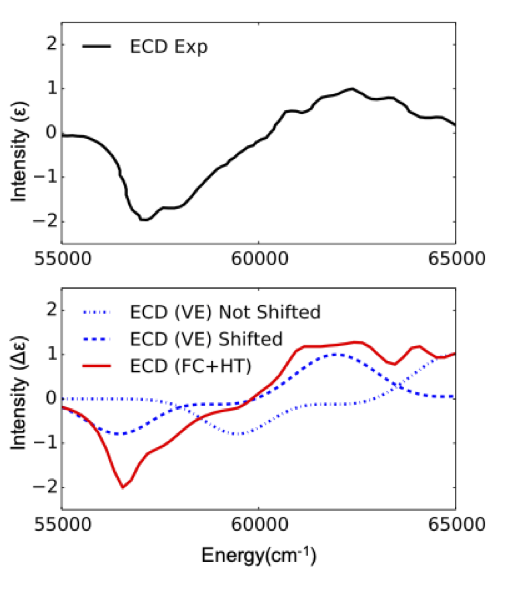
Fig. 6.69 Experimental (black) versus BP86/TDDFT (VE, blue and FC+HT red) ECD spectra for C3H6O molecule
6.18.8.3. Computation of CP-FLUOR vs CP-PHOS spectra. The case of \(C_{3}H_{6}O\).
Following the strategy described for the computation of PL (Fluorescence (PF) of Phosphorescence (PP)) spectra in the case of \(C_{3}H_{6}O\) one can also access the respective CPL and CPP spectra.
For this one needs to compute the hessian of the 1st excited singlet (ES1) and triplet states respectively (ET0) according to the following inputs
!BP86 DEF2-SVP TIGHTSCF OPT FREQ

%TDDFT
NROOTS 10
IROOT 1
IMULT 1
END

* xyzfile 0 1 c3h6o_opt_freq.xyz
and
!BP86 DEF2-SVP TIGHTSCF OPT FREQ

%TDDFT
NROOTS 10
IROOT 1
IMULT 3
SOCGRAD TRUE
TRIPLETS TRUE
END

* xyzfile 0 3 c3h6o_opt_freq.xyz
Then one can setup the respective PL and CPL inputs as:
PF:
!BP86 DEF2-SVP TIGHTSCF

%TDDFT
NROOTS 10
IROOT 1
IMULT 1
END

%ESD
ESDFlag FLUOR
GSHESSIAN "C3H6O_opt.hess"
PRINTLEVEL 2
DOHT TRUE
LINEW 500
SPECRANGE 40000, 70000
END

* xyzfile 0 1 c3h6o_opt_freq.xyz
CPF:
!BP86 DEF2-SVP TIGHTSCF

%TDDFT
NROOTS 10
IROOT 1
IMULT 1
END

%ESD
ESDFlag CPF
GSHESSIAN "C3H6O_opt.hess"
PRINTLEVEL 2
DOHT TRUE
LINEW 500
SPECRANGE 40000, 70000
END

* xyzfile 0 1 c3h6o_opt_freq.xyz
PP:
!BP86 DEF2-SVP TIGHTSCF

%TDDFT
NROOTS 10
IROOT 1
IMULT 3
DoSOC true
TRIPLETS TRUE
SOCGRAD TRUE
END

%ESD
ESDFlag PHOSP
GSHESSIAN "C3H6O_opt_freq.hess"
TSHESSIAN "C3H6O_et0.hess"
PRINTLEVEL 2
DELE 62313
DOHT TRUE
LINEW 500
TEMP  295
SPECRANGE 40000, 70000
END

* xyzfile 0 1 C3H6O_opt.xyz
CPP:
!BP86 DEF2-SVP TIGHTSCF

%TDDFT
NROOTS 10
IROOT 1
IMULT 3
DoSOC true
TRIPLETS TRUE
SOCGRAD TRUE
END

%ESD
ESDFlag CPP
GSHESSIAN "C3H6O_opt_freq.hess"
TSHESSIAN "C3H6O_et0.hess"
PRINTLEVEL 2
DELE 62313
DOHT TRUE
LINEW 500
TEMP  295
SPECRANGE 40000, 70000
END

* xyzfile 0 1 C3H6O_opt.xyz
The results are summarized in Figure Fig. 6.70
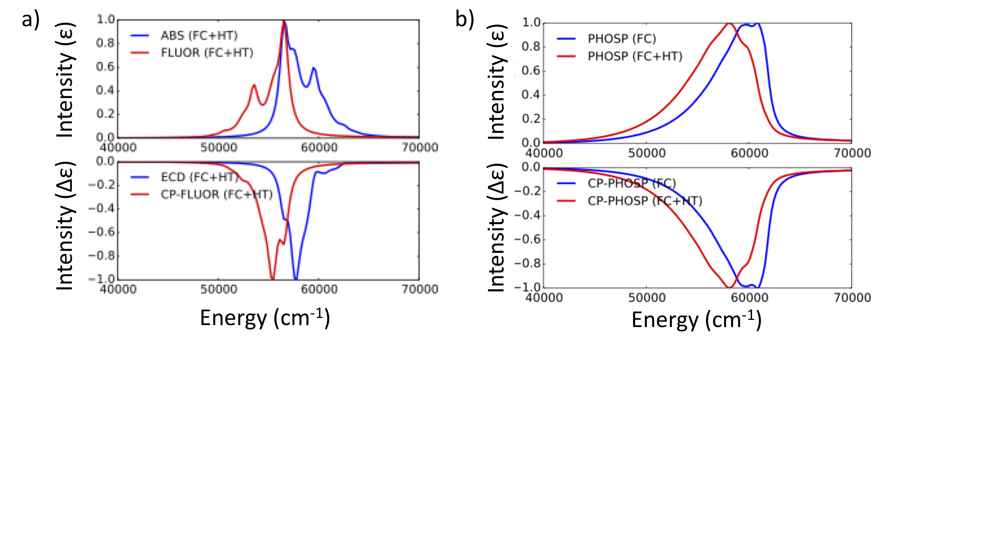
Fig. 6.70 a) Computed ABS and ECD (in blue) and Florescence and CPF (in red) under FC+HT vibronic coupling schemes b) Computed Phosphorescence and CPP under FC (in blue ) and FC+HT (in red) vibronic coupling schemes
6.18.8.4. Use of ABS, ECD PL and CPL as a routine analysis computational tools
Having at hand the possibility to compute the above spectroscopic properties quartet.
Consisting of Absorption, ECD, Luminescent/Emission and CPL spectroscopies creates an arsenal
of useful analysis computational tools. Let us consider a practical example from the
the N- bridged triarylamine heterohelicenoid chiral family of molecules, which are known to be
very good CPL emitters in the CPL community. [186]
Namely the R-, L- isomers of oxygen-bridged diphenylnaphthylamine for which
both ABS ECD, PL and CPL experimental spectra are available [635]
In a first step one needs to compute to calculate the ECD and CPL spectra, this implies that one needs to optimize the ground state (GS) geometry and at least the GS hessian of both isomers, (see examples in Fluorescence Rates and Spectrum and Vibration effects on ECD spectra). Lets suppose that we have generated the GSHessian file R_OptFreq.hess file for the R-isomer Then one can employ the ESD to calculate the Absorption, ECD, Fluorescence and CPL (CPluorescecne) as follows.
For Absorption or ECD spectra a representative input is given by:
! PBE0 def2-TZVP def2/J def2-TZVP VeryTightSCF PAL8
%MaxCore 5120

%TDDFT NROOTS 5
       End

%ESD   ESDFlag     ABS or ECD
       GSHessian  "R_diphenylnaphthylamine_OptFreq.hess"
       DoHT        True
       Lines       Gauss
       InLineW     500
       STATES      1,2,3,4,5
       End

*xyz 0 1
C           0.51103659781880     -1.54799809918165     -0.46957711710367
C          -0.67682083480241     -2.19898547218227     -0.76456508506476
C           1.59698089595014     -2.23913762447750      0.04536520831045
C           1.49004594789848     -3.60107534512753      0.24696861333386
C          -0.75027591609003     -3.56343872947031     -0.57021086417552
C           0.33765559244610     -4.27346122451739     -0.10341675327345
N           0.21984508391204     -5.66346290617628      0.07289766826829
O           2.52716581975956     -4.28847037580032      0.82258958688483
C           2.54101738078760     -5.65282427633174      0.65190453446035
C           1.43184892145219     -6.36105379222857      0.25831057061542
C           3.77147940706722     -6.27965254373750      0.89001683729049
C           3.89719111077242     -7.62085864051752      0.70851807608572
C           1.58029288205151     -7.74060974139699     -0.06585842329724
C           2.81811727341129     -8.37881977445777      0.20527726022176
O          -1.91500963727701     -4.25152600059560     -0.80702339426568
C          -2.13250715287481     -5.31470429649343      0.04909464399864
C          -1.05242665026610     -6.06056594251354      0.52598562255970
C          -3.42444532048472     -5.61905191519688      0.41037068048411
C          -3.66399173496155     -6.68754268865431      1.26210310826770
C          -1.29901325564529     -7.09753540866930      1.41085143603056
C          -2.60176522746573     -7.41491597190339      1.76502960065907
H          -4.22973438581776     -5.01558835826860      0.01489276124005
H          -4.67873778203345     -6.93777656190575      1.53843511994436
H          -0.47290745868829     -7.66765085401275      1.80929822862278
H          -2.77926863803574     -8.23774715258380      2.44386581691750
H           0.58624233693590     -0.48095844424254     -0.62562692246504
H           2.51652973024519     -1.73662559987765      0.30924801794967
H          -1.54272285055189     -1.66670869597130     -1.13102495882678
H           4.59563142014220     -5.66684912938550      1.22771972849030
H           4.83828110533620     -8.11484947410606      0.91089239524435
C           0.56233992156145     -8.49575213625774     -0.69451663429121
C           2.96252715039542     -9.75415434575818     -0.08347675768224
C           0.74593486971180     -9.81550692161063     -0.98488391710801
C           1.95147468552282    -10.46257812809982     -0.65848843248314
H          -0.36538542100730     -8.01665224889233     -0.96504181763392
H          -0.04242675451776    -10.36879326589460     -1.47770458618347
H           2.07785937833070    -11.51320955617077     -0.88255640316097
H           3.90687057621082    -10.23141194413179      0.14665882143507
*
For Fluorescence or CP Fluorescence spectra a representative input is given by:
! PBE0 def2-TZVP def2/J def2-TZVP VeryTightSCF PAL8
%MaxCore 5120

%TDDFT NROOTS 5
       End

%ESD   ESDFlag     FLUOR or CPF
       GSHessian  "R_diphenylnaphthylamine_OptFreq.hess"
       DoHT        True
       Lines       Gauss
       InLineW     500
       STATES      1,2,3,4,5
       End

*xyz 0 1
C           0.51103659781880     -1.54799809918165     -0.46957711710367
C          -0.67682083480241     -2.19898547218227     -0.76456508506476
C           1.59698089595014     -2.23913762447750      0.04536520831045
C           1.49004594789848     -3.60107534512753      0.24696861333386
C          -0.75027591609003     -3.56343872947031     -0.57021086417552
C           0.33765559244610     -4.27346122451739     -0.10341675327345
N           0.21984508391204     -5.66346290617628      0.07289766826829
O           2.52716581975956     -4.28847037580032      0.82258958688483
C           2.54101738078760     -5.65282427633174      0.65190453446035
C           1.43184892145219     -6.36105379222857      0.25831057061542
C           3.77147940706722     -6.27965254373750      0.89001683729049
C           3.89719111077242     -7.62085864051752      0.70851807608572
C           1.58029288205151     -7.74060974139699     -0.06585842329724
C           2.81811727341129     -8.37881977445777      0.20527726022176
O          -1.91500963727701     -4.25152600059560     -0.80702339426568
C          -2.13250715287481     -5.31470429649343      0.04909464399864
C          -1.05242665026610     -6.06056594251354      0.52598562255970
C          -3.42444532048472     -5.61905191519688      0.41037068048411
C          -3.66399173496155     -6.68754268865431      1.26210310826770
C          -1.29901325564529     -7.09753540866930      1.41085143603056
C          -2.60176522746573     -7.41491597190339      1.76502960065907
H          -4.22973438581776     -5.01558835826860      0.01489276124005
H          -4.67873778203345     -6.93777656190575      1.53843511994436
H          -0.47290745868829     -7.66765085401275      1.80929822862278
H          -2.77926863803574     -8.23774715258380      2.44386581691750
H           0.58624233693590     -0.48095844424254     -0.62562692246504
H           2.51652973024519     -1.73662559987765      0.30924801794967
H          -1.54272285055189     -1.66670869597130     -1.13102495882678
H           4.59563142014220     -5.66684912938550      1.22771972849030
H           4.83828110533620     -8.11484947410606      0.91089239524435
C           0.56233992156145     -8.49575213625774     -0.69451663429121
C           2.96252715039542     -9.75415434575818     -0.08347675768224
C           0.74593486971180     -9.81550692161063     -0.98488391710801
C           1.95147468552282    -10.46257812809982     -0.65848843248314
H          -0.36538542100730     -8.01665224889233     -0.96504181763392
H          -0.04242675451776    -10.36879326589460     -1.47770458618347
H           2.07785937833070    -11.51320955617077     -0.88255640316097
H           3.90687057621082    -10.23141194413179      0.14665882143507
*
The results are summarized in Figure Fig. 6.71
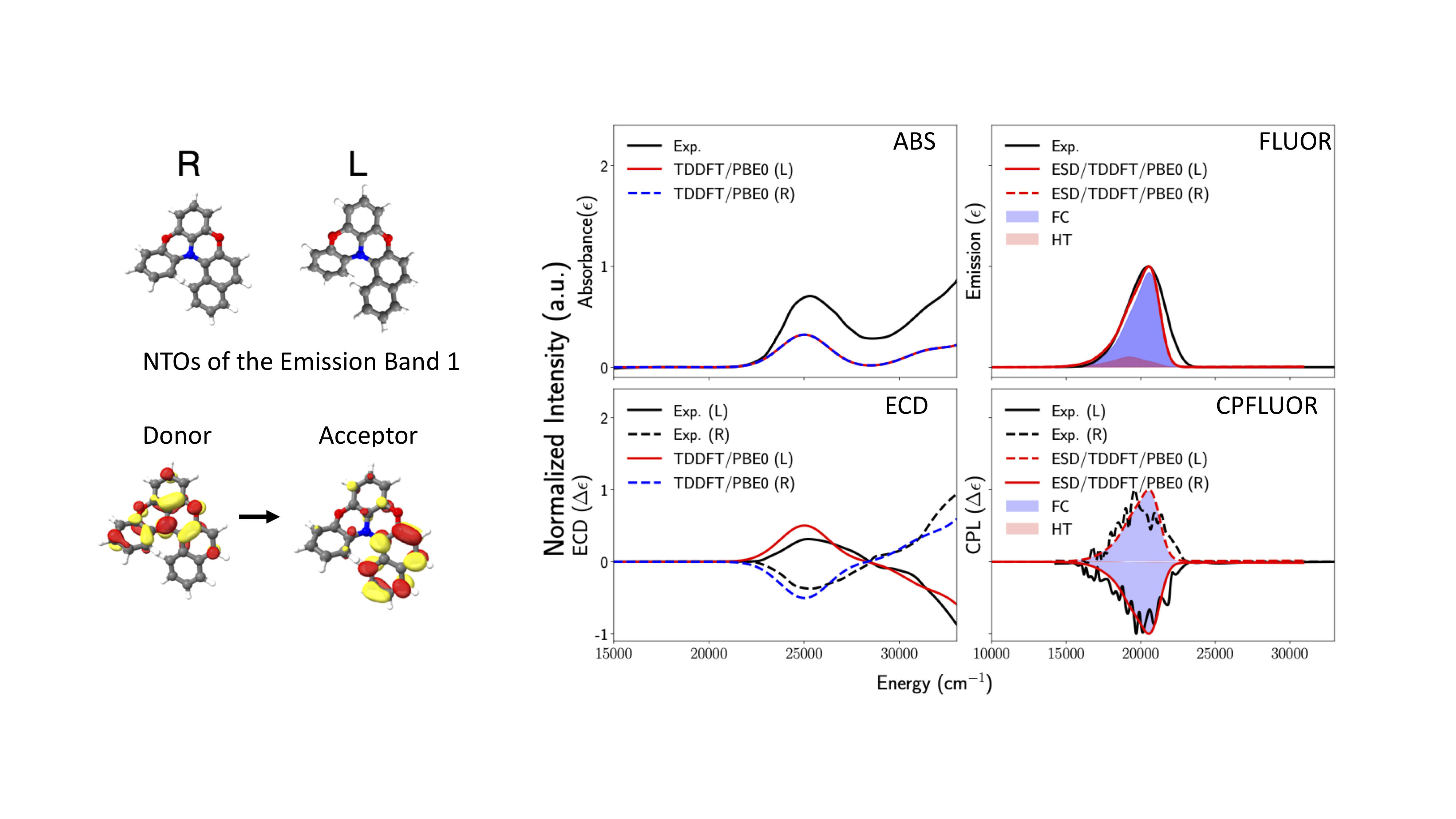
Fig. 6.71 Black Experimental vs Calculated ABS, ECD, Fluorescence and CPF spectra for R- (in blue) and L- (in red) isomers of diphenylnaphthylamine under FC+HT vibronic coupling schemes of the \(\pi\rightarrow\pi^*\) transition located at 25000 \(cm^{-1}\).
6.18.9. Magnetic Circular Dichroism (unpublished)
6.18.9.1. General Aspects
By applying a quasi-degenerate perturbative theory, similar to the inclusion of spin-orbit coupling effects in the phosphorescence calculations, the effect of an external magnetic field may be included in the representation of the quantum states [268]. As a result, the differential absorption of left and right circularly polarized light may be computed to obtain the vibrationally-corrected magnetic circularly dichroism spectrum. The input for the calculation is similar to the absorption case described above; nevertheless, ESD(MCD) should be used. Additionally, the intensity of the external magnetic field “B” (in Gauss) should be included, and a Lebedev grid for a semi-numerical molecular orientational average should be selected.
The method is only available with an electronic structure generated by TDDFT. The calculation supports the inclusion of Herzberg-Teller effects by setting DOHT TRUE, the ground state Hessian needs to be provided similarly to the absorption case, while the excited state Hessian can be provided or computed under a no external magnetic field approximation. An input example is:
!B3LYP DEF2-TZVP TIGHTSCF ESD(MCD)

%TDDFT NROOTS 40
       TDA FALSE
END

%ESD    GSHESSIAN "pbq.hess"
        Hessflag AHAS
        DOHT    TRUE
        STATES 1
        B 50000.0
END

* xyzfile 0 1 pbq.xyz
Similarly, to the ESB(ABS) calculation the MCD spectrum is saved in a BASENAME.MCD file as:
Energy          TotalSpectrum           IntensityFC             IntensityHT
4817.11         -6.324671e-05           -4.528264e-06           -5.871844e-05
5026.55         -6.717718e-05           -4.809014e-06           -6.236816e-05
5235.99         -7.126386e-05           -5.100843e-06           -6.616302e-05
5445.43         -7.551756e-05           -5.404513e-06           -7.011304e-05
5654.87         -7.994996e-05           -5.720850e-06           -7.422911e-05
5864.31         -8.457379e-05           -6.050750e-06           -7.852304e-05
...
6.18.10. Tips, Tricks and Troubleshooting
Currently, the ESD module works optimally with TD-DFT (Sec. Excited States Calculations), but also with ROCIS (Sec. Excited States with RPA, CIS, CIS(D), ROCIS and TD-DFT), EOM/STEOM (Sec. Excited States with EOM-CCSD and Sec. Excited States with STEOM-CCSD) and CASSCF/NEVPT2 (Sec. Complete Active Space Self-Consistent Field Method and Sec N-Electron Valence State Perturbation Theory (NEVPT2)). Of course you can use any two Hessian files and input a custom DELE and TDIP obtained from any method (see Sec. More on the Excited State Dynamics module), if your interested only in the FC part.
If you request for the HT effect, calculating absorption or emission, you might encounter phase changes during the displacements during the numerical derivatives of the transition dipole moment. There is a phase correction for TD-DFT and CASSCF, but not for the other methods. Please be aware that phase changes might lead to errors.
Please check the K*K value if you have trouble. When it is too large (in general larger than 7), a warning message is printed and it means that the geometries might be too displaced and the harmonic approximation might fail. You can try removing some modes using TCUTFREQ or use a different method for the ES PES.
If using DFT, the choice of functional can make a big difference on the excited state geometry, even if it is small on the ground state. Hybrid functionals are much better choices than pure ones.
In CASSCF/NEVPT2, the IROOT flag has a different meaning from all other modules. In this case, the ground state is the IROOT 1, the first excited state is IROOT 2 and so on. If your are using a state-averaged calculation with more than one multiplicity, you need also to set an IMULT to define the right block, IMULT 1 being the first block, IMULT 2 the second and etc.
If using NEVPT2 the IROOT should be related to the respective CASSCF root, don’t consider the energy ordering after the perturbation.
After choosing any of the HESSFLAG options, a BASENAME.ES.hess file is saved with the geometry and Hessian for the ES. If derivatives with respect to the GS are calculated, a BASENAME.GS.hess is also saved. Use those to avoid recalculating everything over and over. If you just want to get an ES PES, you can set WRITEHESS TRUE under
Although in principle more complete, the AH is not NECESSARILY better, for we rely on the harmonic approximation and large displacements between geometries might lead to errors. In some cases the VG, AHAS and so one might be better options.
If you use these .hess files with derivatives over normal modes in one coordinate system, DO NOT MIX IT with a different set of coordinates later! They will not be converted.
Sometimes, low frequencies have displacements that are just too large, or the experimental modes are too anharmonic and you might want to remove them. It is possible to do that setting the TCUTFREQ flag (in cm\(^{-1}\)), and all frequencies below the given threshold will be removed.
If you want to change the parameters related to the frequency calculations, you can do that under %FREQ (Sec. Vibrational Frequencies). The numerical gradient settings are under %NUMGRAD (Sec. Numerical Gradients).
When computing rates, the use of any LINES besides DELTA is an approximation. It is recommended to compute the rate at much smaller lineshape (such as 10 cm\(^{-1}\)) to get a better value, even if the spectrum needs a larger lineshape than that.
When in doubt, try setting a higher PRINTLEVEL. some extra printing might help with your particular problem.