7.15. The Complete Active Space Self-Consistent Field (CASSCF) Module
7.15.1. General Description
The complete active space self-consistent field (CASSCF) method is a special form of a multiconfigurational SCF method and can be thought of as an extension of the Hartree-Fock method. It is a very powerful method to study static correlation effects and a solid basis for MR-CI and MR-PT treatments. It can be applied to the ground state and excited states or averages thereof. The implementation in ORCA is fairly general and reasonably efficient. However, CASSCF calculations are fairly complex and ultimately require a lot of insight from the user in order to be successful. In addition to detailed description here, the manual explores some typical examples in section CASSCF Natural Orbitals as Input for Coupled-Cluster Calculations. Furthermore, the manual is supplemented with a tutorial for CASSCF that covers many practical tips on the calculation design and usage of the program.
The wavefunction. The wavefunction of a given CASSCF state is written as
Here, \(\left| \Psi_I^S \right\rangle\) is the CASSCF \(N\)-electron wavefunction for state \(I\) with total spin S. The set of \(\left| \Phi_k^S \right\rangle\) is a set of configuration state functions (for example linear combination of Slater determinants) each adapted to a total spin \(S\). The expansion coefficients \(C_{kI}\) represent the first set of variational parameters. Each CSF is constructed from a common set of orthonormal molecular orbitals \(\psi_{i} \left({ \mathrm{\mathbf{r} }} \right)\) which are in turn expanded in basis functions \(\psi_{i} \left({ \mathrm{\mathbf{r} }} \right)=\sum\nolimits_\mu{c_{\mu i} \phi_{\mu } \left({ \mathrm{\mathbf{r} }} \right)}\). The MO coefficients \(c_{\mu i}\) form the second set of variational parameters.
The energy. The energy of the CASSCF wavefunction is given by the Rayleigh quotient
and represents an upper bound to the true total energy. However, CASSCF calculations are not designed to provide values for total energy which are close to the exact energy. The purpose of a CASSCF calculation is to provide a qualitatively correct wavefunction, which forms a good starting point for a treatment of dynamic electron correlation.
The CASSCF method is fully variational in the sense that the energy is made stationary with respect to variations in both sets of MO and CI coefficients. At convergence, the gradient of the energy with respect to the MO and CI coefficients vanishes
Orbital spaces. In CASSCF calculations, the MO space is divided into three user defined subspaces:
The “inactive orbitals” are the orbitals which are doubly occupied in all configuration state functions (labels \(i, j, k, l\)).
The “active orbitals” are the orbitals with variable occupation numbers in the various CSFs (labels \(t, u, v, w\)).
The “external orbitals” (labels \(a, b, c, d\))
Note that in older publications, the inactive and active orbitals are distinguished and referred to as “internal” orbitals.
The wavefunction and energy is invariant with respect to unitary transformations within the three subspaces. The special feature of a CASSCF wavefunction is that a fixed number of electrons is assigned to each subspace. The internal subspace is of course completely filled but the CSFs in the active space constitute a full-CI of \(n\)-electrons in \(m\)-orbitals. The CSF list is constructed such, however, that a wavefunction of well defined total spin (and potential space) symmetry results. Such a wavefunction is referred to as a CASSCF(\(n\),\(m\)) wavefunction. The CSF list grows extremely quickly with the number of active orbitals and the number of active electrons (basically factorially). Depending on the system, the limit of feasibility is roughly around \(\sim\)14 active orbitals or about one million CSFs in the active space. Larger active spaces are tractable with approximate CI solver such as the Iterative-Configuration-Expansion CI (ICE-CI) described in Approximate Full CI Calculations in Subspace: ICE-CI or the Density Matrix Renormalization Group (DMRG) discussed in Density Matrix Renormalization Group.[1]
Since the orbitals within the subspaces are only defined up to a unitary transformation, the program needs to make some canonicalization choice.
In ORCA, the final orbitals by default are:
natural orbitals in the active space,
orbitals which diagonalize the CASSCF Fock matrix in the internal space and
orbitals which diagonalize the CASSCF Fock matrix in the external space.
State averaging. In many circumstances, it is desirable to optimize the orbitals not for a single state but for the average of several states. In order to see what is done, the energy for state \(I\) is re-written as:
Here, \(\Gamma_{q}^{p\left( I \right)}\) and \(\Gamma_{qs}^{pr\left( I \right)}\) are the one-and two-particle reduced electron density matrices for this state (labels \(p, q, r, s\) span the internal and active subspaces):
The average energy is simply obtained from averaging the density matrices using arbitrary weights \(w_{I}\) that are user defined but are constrained to sum to unity.
Optimization of CASSCF wavefunctions. In general, except for trivial cases, CASSCF wavefunctions are considerably more difficult to optimize than RHF (or UHF) wavefunctions. The underlying reason is that variations in c and C maybe strongly coupled and the energy functional may have many local minima in (c,C) space. Consequently, the choice of starting orbitals is of really high importance and the choice which orbitals and electrons are included in the active space has decisive influence on the success of a CASSCF study. In general, after transformation to natural orbitals, one can classify the active space orbitals by their occupation numbers which vary between 0.0 and 2.0. In general, convergence problems are almost guaranteed if orbitals with occupation numbers close to zero or close to 2.0 are included in the active space. Occupation numbers between 0.02 and 1.98 are typically very reasonable and should not lead to large convergence problems. The reason for the occurrence of convergence problems is that the energy is only very weakly dependent on rotations between internal and active orbitals if the active orbital is almost doubly occupied and similarly for the rotations between external and weakly occupied active orbitals. However, in some cases (for example in the study of potential energy surfaces) it may not be avoidable to include weakly or almost inactive orbitals in the active space and in these cases the use of the most powerful convergence aids is necessary (vide infra). As in the case of single-determinant wavefunctions (RHF, UHF, RKS, UKS) there are first and second order converging methods available. The first order CASSCF methods require the transformed integrals \((tu|vx)\) with \(x\) belonging to any subspace. This is a very small subspace of the total transformed integral list and is readily held in central storage even for larger calculations. On the other hand, second order CASSCF methods require the integrals \((pq|xy)\) and \((px|qy)\) (\(p,q=\) internal, active; \(x,y=\) any orbital). This is a fairly large set of integrals and their generation is laborious in terms of CPU time and disk storage. Second order CASSCF calculations are therefore more limited in the size of the molecules which can be well treated. It would be possible to basically avoid the integral transformation also in the case of second-order CASSCF calculations and proceed to fully direct calculations. Such calculations may become quite time consuming since there may be a large number of Fock matrix builds necessary.
The augmented Hessian method (Newton-Raphson) solves the eigenvalue problem:
Here, \(\mathrm{\mathbf{g} }\) is the orbital gradient (derivative of the total energy with respect to a non-redundant rotation between two orbitals) and \(\mathrm{\mathbf{H} }\) is the orbital Hessian (second derivative of the energy with respect to two non-redundant orbital rotations). The vector \(\mathrm{\mathbf{t} }\) (in intermediate normalization obtained from the CI like vector) summarizes the rotation angles. The angles are used to define the antisymmetric matrix (\(X_{pq} =-X_{qp}\) is thus the rotation angle between orbitals \(p\) and \(q\)):
which is used to parametrize the unitary matrix \(\mathrm{\mathbf{U} }=\exp \left({\mathrm{\mathbf{X} }} \right)\) which is used to update the orbitals according to:
(where \(\mathrm{\mathbf{c} }\) is an MO coefficient matrix).
Starting orbitals. You cannot be careful enough with your starting
orbitals. What type of initial guess works best depends on the system.
Quite often it is not the magnitude of the initial gradient, but the
similarity between initial and final active orbitals. The CASSCF
tutorial discusses a number of guess options in more detail. Generally
speaking, canonical orbitals HF orbitals from a RHF calculation are not
good choice, as the identification and selection of the active space
orbitals is often difficult. Usually DFT orbitals (quasi-restricted or
RKS) perform better in this respect. Alternatively, if CASSCF orbitals
from a previous run or a close-by geometry are available this is a good
choice. For coordination chemistry complexes, the guess generated with
orca_mergefrag (see the CASSCF tutorial), is probably the best
choice - especially for heave metals. Natural orbitals from a simple
correlation calculation like MP2 or a calculation with the MRCI module
are usually a good choice and easily generated. For example:
#
# First job provides reasonable natural orbitals
#
! RI-MP2 SVP def2-SVP/C

%mp2 natorbs true
     density unrelaxed # or relaxed (more expensive)
     end

* int 0 1
    C  0 0 0 0.00   0.0    0.00
    O  1 0 0 1.20   0.0    0.00
    H  1 2 0 1.10 120.0    0.00
    H  1 2 3 1.10 120.0  180.00
*
Now examine the occupation numbers of the natural orbitals (you will find that in the output of the MP2 part of the calculation):
Natural Orbital Occupation Numbers:
N[  0] =   2.00000000
N[  1] =   2.00000000
N[  2] =   1.98676733
N[  3] =   1.97726840
N[  4] =   1.97500109
N[  5] =   1.96759239
N[  6] =   1.96423113
N[  7] =   1.93719340
N[  8] =   0.05427454
N[  9] =   0.02555886
N[ 10] =   0.02530580
N[ 11] =   0.01358500
N[ 12] =   0.01096092
N[ 13] =   0.01028129
N[ 14] =   0.00702048
N[ 15] =   0.00627820
A rule of thumb is that orbitals with occupation numbers between 1.98 and 0.02 should be in the active space. Thus, in the present case we speculate that a 10 electrons in 8 orbitals active space would be appropriate for the CASSCF of the ground state. Let’s try:
#
# Run a CASSCF calculation for the ground state of H2CO
#
! SVP def2-SVP/C SmallPrint
! moread
%moinp "Test-CASSCF-MP2-H2CO.mp2nat"

%casscf nel        10
        norb        8
	mult        1
        end

* int 0 1
    C  0 0 0 0.00   0.0    0.00
    O  1 0 0 1.20   0.0    0.00
    H  1 2 0 1.10 120.0    0.00
    H  1 2 3 1.10 120.0  180.00
*
If we run that calculation, it converges and produces the following:
MACRO-ITERATION  10:
	--- Inactive Energy E0 = -82.97337099 Eh
	E(CAS)=  -113.889438276 Eh DE=    -0.000000807
	--- Energy gap subspaces: Ext-Act = -0.431   Act-Int = -0.240
	N(occ)=  1.99763 1.99696 1.98360 1.97923 1.94253 0.05958 0.02153 0.01894
	||g|| =      0.000361782 Max(G)=     0.000189613 Rot=9,2
	---- THE CAS-SCF GRADIENT HAS CONVERGED ----
	          --- FINALIZING ORBITALS ---
	---- DOING ONE FINAL ITERATION FOR PRINTING ----
	--- Forming Natural Orbitals
	--- Canonicalize Internal Space
	--- Canonicalize External Space
From which we see that we had two orbitals too many in the active space with occupation numbers very close to two. The presence of barely correlated orbitals (occupation close to 0.0 or 2.0) can cause convergence problems. Their inclusion in the active space does not significantly change the energy and it might better to omit these orbitals from the start.
In the present case, we re-run the CASSCF with 6 active electrons in six orbitals. The result is:
MACRO-ITERATION   2:
	--- Inactive Energy E0 = -101.16144179 Eh
	E(CAS)=  -113.882700257 Eh DE=    -0.012049926
	--- Energy gap subspaces: Ext-Act = -0.411   Act-Int = -0.142
	N(occ)=  1.98172 1.97921 1.94092 0.05983 0.02089 0.01743
	||g|| =      0.052811635 Max(G)=     0.025065586 Rot=19,7
	--- Orbital Update [SuperCI(PT)]
	--- Canonicalize Internal Space
	--- Canonicalize External Space
	--- SX_PT (Skipped TA=0 IT=0): ||X|| =      0.160674186 Max(X)(5,4) =     -0.128053569
	--- SFit(Active Orbitals)

	MACRO-ITERATION   3:
	--- Inactive Energy E0 = -100.78371592 Eh
	E(CAS)=  -113.885011169 Eh DE=    -0.002310912
	--- Energy gap subspaces: Ext-Act = -0.434   Act-Int = -0.199
	N(occ)=  1.98150 1.97909 1.94143 0.05924 0.02108 0.01766
	||g|| =      0.017438409 Max(G)=     0.009231446 Rot=10,4
	--- Orbital Update [SuperCI(PT)]
	--- Canonicalize Internal Space
	--- Canonicalize External Space
	--- SX_PT (Skipped TA=0 IT=0): ||X|| =      0.050337699 Max(X)(6,2) =     -0.033671129
	--- SFit(Active Orbitals)

	MACRO-ITERATION   4:
	--- Inactive Energy E0 = -100.72313195 Eh
	E(CAS)=  -113.885258854 Eh DE=    -0.000247685
	--- Energy gap subspaces: Ext-Act = -0.438   Act-Int = -0.219
	N(occ)=  1.98141 1.97918 1.94178 0.05886 0.02102 0.01776
	||g|| =      0.009726271 Max(G)=     0.004281706 Rot=9,2
	--- Orbital Update [SuperCI(PT)]
	--- Canonicalize Internal Space
	--- Canonicalize External Space
	--- SX_PT (Skipped TA=0 IT=0): ||X|| =      0.031123960 Max(X)(22,9) =      0.015789781
	--- SFit(Active Orbitals)

	MACRO-ITERATION   5:
	--- Inactive Energy E0 = -100.65264536 Eh
	E(CAS)=  -113.885424851 Eh DE=    -0.000165997
	--- Energy gap subspaces: Ext-Act = -0.440   Act-Int = -0.238
	N(occ)=  1.98140 1.97918 1.94202 0.05857 0.02105 0.01776
	||g|| =      0.006606671 Max(G)=     0.003548636 Rot=9,2
	--- Orbital Update [SuperCI(PT)]
	--- Canonicalize Internal Space
	--- Canonicalize External Space
	--- SX_PT (Skipped TA=0 IT=0): ||X|| =      0.019988497 Max(X)(6,2) =     -0.014410848
	--- SFit(Active Orbitals)

	MACRO-ITERATION   6:
	--- Inactive Energy E0 = -100.56070274 Eh
	E(CAS)=  -113.885549550 Eh DE=    -0.000124699
	--- Energy gap subspaces: Ext-Act = -0.440   Act-Int = -0.268
	N(occ)=  1.98138 1.97925 1.94206 0.05849 0.02104 0.01778
	||g|| =      0.004483296 Max(G)=     0.002939015 Rot=9,2
	--- Orbital Update [SuperCI(PT)]
	--- Canonicalize Internal Space
	--- Canonicalize External Space
	--- SX_PT (Skipped TA=0 IT=0): ||X|| =      0.011383690 Max(X)(5,4) =      0.005997355
	--- SFit(Active Orbitals)

	MACRO-ITERATION   7:
	--- Inactive Energy E0 = -100.52522560 Eh
	E(CAS)=  -113.885583124 Eh DE=    -0.000033574
	--- Energy gap subspaces: Ext-Act = -0.437   Act-Int = -0.283
	N(occ)=  1.98132 1.97929 1.94192 0.05861 0.02103 0.01783
	||g|| =      0.002275031 Max(G)=    -0.001215398 Rot=10,4
	--- Orbital Update [SuperCI(PT)]
	--- Canonicalize Internal Space
	--- Canonicalize External Space
	--- SX_PT (Skipped TA=0 IT=0): ||X|| =      0.002106033 Max(X)(19,10) =     -0.001056121
	--- SFit(Active Orbitals)

	MACRO-ITERATION   8:
	--- Inactive Energy E0 = -100.52457962 Eh
	E(CAS)=  -113.885584276 Eh DE=    -0.000001152
	--- Energy gap subspaces: Ext-Act = -0.438   Act-Int = -0.283
	N(occ)=  1.98134 1.97931 1.94184 0.05868 0.02101 0.01781
	||g|| =      0.000752012 Max(G)=    -0.000357510 Rot=13,4
	---- THE CAS-SCF GRADIENT HAS CONVERGED ----
	--- FINALIZING ORBITALS ---
	---- DOING ONE FINAL ITERATION FOR PRINTING ----
	--- Forming Natural Orbitals
	--- Canonicalize Internal Space
	--- Canonicalize External Space

	MACRO-ITERATION   9:
	--- Inactive Energy E0 = -100.52457962 Eh
	--- All densities will be recomputed
	E(CAS)=  -113.885584276 Eh DE=    -0.000000000
	--- Energy gap subspaces: Ext-Act = -0.858   Act-Int = -0.283
	N(occ)=  1.98172 1.97932 1.94207 0.05845 0.02100 0.01743
	||g|| =      0.000752012 Max(G)=    -0.000327367 Rot=12,4
	--------------
	CASSCF RESULTS
	--------------

	Final CASSCF energy       : -113.885584276 Eh   -3098.9843 eV
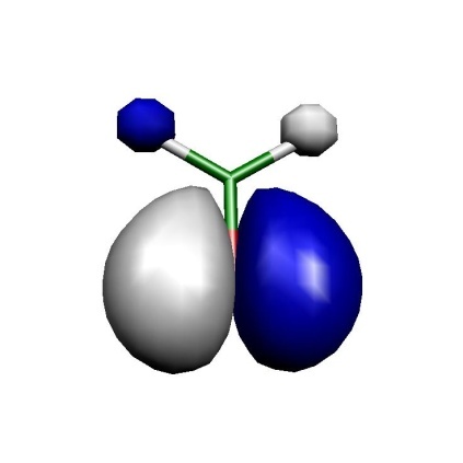
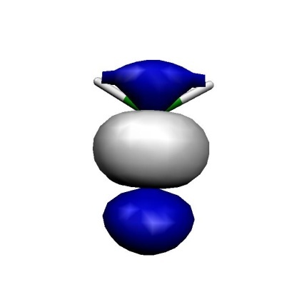
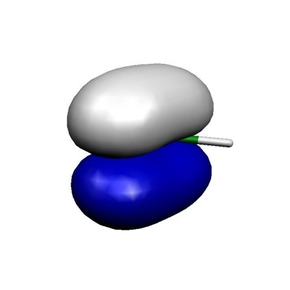
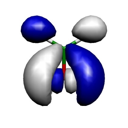
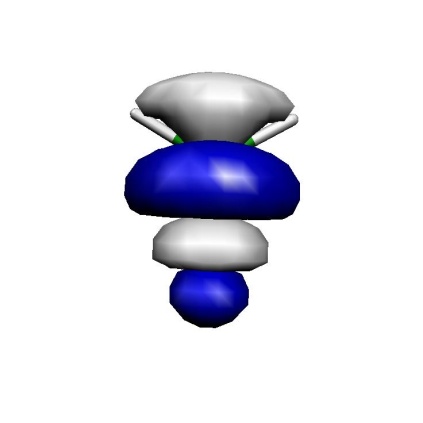
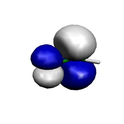
The calculation converges very quickly and the occupation numbers show you that all of these orbitals are actually needed in the active space. The omission of the two orbitals from the active space came at an increase of the energy by \(\sim\)4 mEh which seems to be tolerable. Let’s look what we have in the active space in figure Fig. 7.4.
 MO5
MO5
 MO6
MO6
 MO7
MO7
 MO10
MO10
 MO9
MO9
 MO8
MO8
Fig. 7.4 Orbitals of the active space for the CASSCF(6,6) calculation of H\(_2\)CO.
Thus, we can see that we got a fairly nice result: our calculation has correlated the in-plane oxygen lone pair, the C-O \(\sigma\) and the C-O \(\pi\) bond. For each strongly occupied bonding orbital, there is an accompanying weakly occupied antibonding orbital in the active space that is characterized by one more node. In particular, the correlating lone pair and the C-O \(\sigma^{\ast }\) orbital would have been hard to find with any other procedure than the one chosen based on natural orbitals. We have now done it blindly and looked at the orbitals only after the CASSCF — a better approach is normally to look at the starting orbitals before you enter a potentially expensive CASSCF calculation. If you have bonding/antibonding pairs in the active space plus perhaps the singly-occupied MOs of the system you probably have chosen a reasonable active space.
We can play the game now somewhat more seriously and optimize the geometry of the molecule using a reasonable basis set:
! def2-TZVP def2-TZVP/C SmallPrint Opt
! moread
%moinp "Test-CASSCF-MP2-H2CO.mp2nat"

%casscf nel         6
        norb        6
        end

* int 0 1
    C  0 0 0 0.00   0.0    0.00
    O  1 0 0 1.20   0.0    0.00
    H  1 2 0 1.10 120.0    0.00
    H  1 2 3 1.10 120.0  180.00
*
and get:
---------------------------------------------------------------------------
    Redundant Internal Coordinates

    --- Optimized Parameters ---
    (Angstroem and degrees)

    Definition                    OldVal   dE/dq     Step     FinalVal
    ----------------------------------------------------------------------------
    1. B(O   1,C   0)                1.2101  0.000259 -0.0002    1.2100
    2. B(H   2,C   0)                1.0942 -0.000029  0.0001    1.0943
    3. B(H   3,C   0)                1.0942 -0.000029  0.0001    1.0943
    4. A(O   1,C   0,H   3)          122.07  0.000023   -0.00    122.07
    5. A(H   2,C   0,H   3)          115.85 -0.000046    0.01    115.86
    6. A(O   1,C   0,H   2)          122.07  0.000023   -0.00    122.07
    7. I(O   1,H   3,H   2,C   0)     -0.00 -0.000000    0.00     -0.00
    ----------------------------------------------------------------------------
Let us compare to MP2 geometries (this job was actually run first):
! RI-MP2 def2-TZVP def2-TZVP/C Opt

%mp2 natorbs true
     end

* int 0 1
    C  0 0 0 0.00   0.0    0.00
    O  1 0 0 1.20   0.0    0.00
    H  1 2 0 1.10 120.0    0.00
    H  1 2 3 1.10 120.0  180.00
*
-------------------------------------------------------------------------
                         Redundant Internal Coordinates

                          --- Optimized Parameters ---
                            (Angstroem and degrees)

        Definition                    OldVal   dE/dq     Step     FinalVal
    ----------------------------------------------------------------------------
     1. B(O   1,C   0)                1.2127  0.000374 -0.0002    1.2125
     2. B(H   2,C   0)                1.0991 -0.000031  0.0001    1.0992
     3. B(H   3,C   0)                1.0991 -0.000031  0.0001    1.0992
     4. A(O   1,C   0,H   3)          121.77  0.000023   -0.00    121.77
     5. A(H   2,C   0,H   3)          116.45 -0.000046    0.01    116.46
     6. A(O   1,C   0,H   2)          121.77  0.000023   -0.00    121.77
     7. I(O   1,H   3,H   2,C   0)     -0.00 -0.000000    0.00     -0.00
    ----------------------------------------------------------------------------
The results are actually extremely similar (better than 1 pm agreement). Compare to RHF:
---------------------------------------------------------------------------
                         Redundant Internal Coordinates

                          --- Optimized Parameters ---
                            (Angstroem and degrees)

        Definition                    OldVal   dE/dq     Step     FinalVal
    ----------------------------------------------------------------------------
     1. B(O   1,C   0)                1.1784 -0.000164  0.0001    1.1785
     2. B(H   2,C   0)                1.0921  0.000010 -0.0000    1.0921
     3. B(H   3,C   0)                1.0921  0.000010 -0.0000    1.0921
     4. A(O   1,C   0,H   3)          121.93 -0.000003   -0.00    121.93
     5. A(H   2,C   0,H   3)          116.13  0.000005    0.00    116.13
     6. A(O   1,C   0,H   2)          121.93 -0.000003   -0.00    121.93
     7. I(O   1,H   3,H   2,C   0)      0.00  0.000000   -0.00     -0.00
    ----------------------------------------------------------------------------
Thus, one can observe that the correlation brought in by CASSCF or MP2 has an important effect on the C\(=\)O distance (\(\sim\)4 pm), while the rest of the geometry is not much affected.
More on the technical use of the CASSCF program.
The most elementary input information which is always required for CASSCF calculations is the specification of the number of active electrons and orbitals.
%casscf nel  4  # number of active space electrons
        norb 6  # number of active orbitals
        end
The CASSCF program in ORCA can average states of several multiplicities. The multiplicities are given as a list. For each multiplicity the number of roots should be specified:
%casscf mult   1,3 # here: multiplicities singlet and triplet

        nroots 4,2 # four singlets, two triplets
        end
If the symmetry handling in ORCA is enabled (! UseSym) each
multiplicity block must have an irreducible representation assigned.
Numbers corresponding to the “irrep” within a given symmetry are
printed in the output of ORCA.
%casscf mult   1,3 # here: multiplicities singlet and triplet
        irrep  0,1 # here: irrep for each mult. block (mandatory!)
        nroots 4,2 # four singlets, two triplets
Several roots and multiplicities usually imply a state average CASSCF (SA-CASSCF) calculation. Note that the program by default chooses equal weights for the multiplicity blocks. Roots within a given block have equal weight. Users can define a custom weighting scheme for the multiplicity blocks and roots:
%casscf mult 1,3   # here: multiplicities singlet and triplet
        nroots 4,2  # four singlets, two triplets
        bweight 2,1 # singlets and triplets weighted 2:1
        weights[0] = 0.5,0.2,0.2,0.2 # singlet weights
        weights[1] = 0.7,0.3         # triplet weights
        end
The program automatically normalizes these weights such that the sum
over all weights is unity. If convergence on an excited state is desired
then the weights[0] array may look like 0.0,0.0,1.0 (this would
optimize the orbitals for the third excited state. If several states
cross during the orbital optimization this will ultimately cause
convergence problems.
We note passing that the converged orbitals of the state averaged
procedure are a compromise for the set of states. ORCA by default only
prints the SA-CASSCF gradient norm. State-specific gradients are
summarized at the end of the calculation with the keyword PrintGState.
%casscf
  ...
  printgstate true # optional printing of the state-specific orbital gradients
end
Orbital optimization methods. In the following we discuss the
available options for orbital optimization. A number of convergence
problems can be resolved changing the guess orbitals. The following
keywords are optional and should only be used facing severe convergence
difficulties. Aside from the SuperCI_PT (default),[459]
several orbital optimization methods (list below) are implemented.
# Keywords to be used as Orbstep/Switchstep
SuperCI_PT  # perturbative SuperCI (first order)
SuperCI     # SuperCI (first order)
DIIS        # DIIS (first order)
KDIIS       # KDIIS (first order)
SOSCF       # approx. Newton-Raphson (first order)
NR          # augmented Hessian Newton-Raphson
            # unfolded two-step procedure
            # - still not true second order
The different convergers have different strengths. First order method
are cheap but typically require more iterations compared to second order
methods. When the gradient is far off from convergence the program uses
the converger defined as orbstep while close to convergence the
switchstep is used. The actual criteria for switchstep are defined
with the keywords SwitchConv and SwitchIter.
%casscf
  OrbStep    SuperCI # or any other from the list above
  SwitchStep DIIS    # or any other from the list above

  SwitchConv 0.03 # gradient at which to switch
  SwitchIter 15   # iteration at which the switch takes place
                  # irrespective of the gradient

  MaxIter     75  # Maximum number of macro-iterations
end
Picking a convergence strategy, the program has to balance speed and
robustness. The default strategy uses the SuperCI_PT as converger for
orbstep and switchstep.[459] This approach determines
the elements \(X_{pq}\) of the anti-Hermitean matrix used in the orbital
update according to
from first order perturbation theory using the Dyall-Hamiltonian
[238] in zeroth order and a first-order perturbed wave
function given as \(\Psi^{(1) }=\sum_{pq}\Psi_p^q X_{qp}\) where the
\(\Psi_p^q\) represent singly excited functions obtained from the CASSCF
wave function by excitation from orbital \(\psi_p\) to orbital \(\psi_q\).
The SuperCI_PT is robust with respect to orbitals that are exactly
doubly occupied or empty. Rotations with orbital close to this critical
occupations can further be eliminated with the keyword DThresh
(default=1e-6). However, the method is quiet aggressive in the orbital
optimization. In some cases, such as basis set projection or PATOM
guess (intrinsic basis set projection), the program might pick a
step-size that is too big. Then restricting the step-size via the
keyword MaxRot (default=0.2) might be useful. The keywords DThresh
and MaxRot described below are specific to SuperCI_PT. For many
users, MaxRot is less palpable than level shifting. Therefore, the
present version allows level shifts as well. In contrast to other
convergers, level shifts are not needed and highly discouraged. With
the exception of GradScaling (vide infra), other damping techniques
described further below do not apply to the SuperCI_PT.
MaxRot 0.05  # cap stepsize for SuperCI_PT
DThresh 1e-6 # thresh for critical occupation
In case of convergence problems with the default settings, it is
recommended to try the combination of orbstep SuperCI and
switchstep DIIS, which in conjuction with a large level shift (2 Eh),
which may be immediately successful. The proposed scheme typically
requires more iterations. Moreoever, in contrast to the SuperCI(PT), the
SuperCI, DIIS and KDIIS should not be used when the active
orbitals have an occupation of exactly 2.0 or 0.0! The DIIS may
sometimes converge slowly or “trail” towards the end such that real
convergence is never reached. The KDIIS [452, 453] — based
on perturbation theory — is an approximation to the regular DIIS
procedure avoiding redundant rotations. Both DIIS schemes avoid linear
dependencies in the expansion space.
MaxDIIS    15    # max. no of DIIS vectors to keep
DIISThresh 1e-7  # overlap criteria for linear dependency
The combination of SuperCI and DIIS (switchstep) is particularly
suited to protect the active space composition. Adjusting the level
shift will do the job. Here, level shift is the single most important
lever to control convergence.
# default = dynamic level-shifting based on Ext-Act, Int-Act
ShiftUp      2.0   # static up-shift the virtual orbitals
ShiftDn      2.0   # static down-shift the internal orbitals
MinShift     0.6   # minimum separation subspaces
Level-shift is particularly important if the active, inactive and
virtual orbitals overlap in their orbital energies. The energy
separation of the subspaces is printed in the output. Ideally, the
entries Ext-Act and Act-Int should be positive and larger than 0.2
Eh. This will help the program to preserve your active space composition
throughout the iterations. If no shift is specified in the input, ORCA
will choose a level-shift to guarantee an energy separation between the
subspaces (MinShift).
E(CAS)=  -230.590325053 Eh DE=    -0.000798832
	--- Energy gap subspaces: Ext-Act = -0.244   Act-Int = -0.002
	--- current l-shift: Up(Ext-Act) = 0.54   Dn(Act-Int) = 0.30
In difficult cases the use of the Newton-Raphson method (NR) is
recommended even if each individual iteration is considerably more
expensive. It is strong towards the end but it would be a waste to start
orbital optimization with the expensive NR method since its radius of
quadratic convergence is quite small. The computationally cheaper
alternative is the SOSCF procedure belonging to the family of
quasi-Newton updates.
Keep in mind that the Newton-Raphson is designed for optimization on a convex surface (Hessian is semidefinite). If the NR is switched on too early, there is a good chance that this condition is not fulfilled. In this case the program will complain about negative eigenvalues or diagonal elements of the Hessian as can be seen in the snippet below. The next optimization step is large and unpredictable. It is a wildcard that can get you closer to convergence or immediate divergence of the CASSCF procedure.
||g|| =      0.771376945 Max(G)=     0.216712933 Rot=140,53
	--- Orbital Update [        NR]
	Warning:  NEGATIVE diagonal element D(81,53)=    -4.733590
	Warning:  NEGATIVE diagonal element D(82,53)=    -4.737955
	...
For larger system, the augmented Hessian equations are solved iteratively (NR iterations). The augmented Hessian is considered solved when the residual norm, \(<r|r>\), is small enough. Aside from the overall CASSCF convergence, negative eigenvalues affect these NR iterations.
--- Orbital Update [        NR]
	AugHess Tolerance (auto): Tol= 1.00e-07
	AUGHESS-ITER   0: E=    -0.174480747 <r|r>=      0.558679452
	AUGHESS-ITER   1: E=    -0.308672359 <r|r>=      0.468254671
	AUGHESS-ITER   2: E=    -0.434272813 <r|r>=      0.286305469
	AUGHESS-ITER   3: E=    -0.439149451 <r|r>=      0.286514628
	AUGHESS-ITER   4: E=    -0.605787445 <r|r>=      0.191691955
	AUGHESS-ITER   5: E=    -0.607766529 <r|r>=      0.310450670
	AUGHESS-ITER   6: E=    -0.611674930 <r|r>=      0.141402593
	AUGHESS-ITER   7: E=    -0.623145299 <r|r>=      0.394505306
	AUGHESS-ITER   8: E=    -0.658410333 <r|r>=      0.166915094
	AUGHESS-ITER   9: E=    -0.790571374 <r|r>=      4.722929453
	AUGHESS-ITER  10: E=    -0.790590554 <r|r>=      4.716012014
	AugHess: No convergence in the Davidson procedure
	...
There are a number of refined NR settings that influence the convergence
behavior on a non-convex energy surface. We mention the keywords for
completeness and dis-encourage from changing the default settings. If
overall convergence cannot be changed due to negative eigenvalues, it is
recommended to delay the NR switchstep (switchconv, switchiter). This
will require some trial and error, since the curvature of the surface is
a priori not know.
%casscf
  ...
  aughess
    Solver   0       # Davidson (default)
    1       # Pople (pure NR steps)
    2       # DIIS
    MaxIter 35       # max. no. of CI iters.
    MaxDim  35       # Davidson expansion space
    MaxDIIS  12      # max. number of DIIS vectors
    UseSubMatrixGuess true # diag a submatrix of the Hessian
    # as an initial guess
    NGuessMat 512   # size of initial guess matrix (part of
    # the Hessian exactly diagonalized)
    ExactDiagSwitch 512 # up to this dimension the Hessian
    # is exactly diagonalized (small problems)
    PrintLevel 1     # amount of output during AH iterations
    Tol    1e-6      # convergence tolerance
    Compress true    # use compressed storage
    DiagShift 0.0    # shift of the diagonal elements of the
    # Hessian
    UseDiagPrec true # use the diagonal in updating
    SecShift 1e-4     # shift the higher roots in the Davidson
    # secular equations
    UpdateShift 0.5  # shift of the denominator in the
    # update of the AH coefficients
  end
end
In general, convergence is strongly influenced by numerical noise, especially in the final iterations. One source of numerical noise is the incremental Fock build. Thus, it can help to enforce more frequent full Fock matrix formation.
ResetFreq 1 # reset frequency for direct SCF
If the orbital change in the active space is small, the active Fock matrix in ORCA is approximated using the density matrix from the previous cycle saving a second Fock matrix build. However, this approximation might also be a source of numerical instability. The threshold “SwitchDens” can be set to zero to enable the exact build. The program default starts with a rather large value (1e-2) and will reduce this parameter automatically when necessary.
switchdens 0.0001 # ~gtol * 0.1
In all of the implemented orbital optimization schemes the step-size
correlates with the gradient-norm. A constant damping factor can be set
with the keyword GradScaling. Note, damping and level shifting
techniques are not recommended for the default converger (SuperCI_PT).
GradScaling 0.5 # constant damping in all steps
There are situations when the active space has been chosen carefully,
but the initial gradient is still far off. To keep the “good” active
space, we can suppress all rotation but the inactive-external ones until
the gradient-norm is small enough to continue safely. The threshold can
be set with FreezeIE keyword. Once the components of the gradient in
the inactive-external direction have a weight of less than FreezeIE,
all constraints are lifted. ORCA by default freezes active rotations if
the total gradient norm is larger than 1.0 and the active rotations have
a weight of less than 5%. The feature can be turned off setting the
threshold to zero.
Similarly, rotations of the almost doubly occupied orbitals with the
inactive orbitals can be damped using the threshold FreezeActive.
Rotations of this type are damped as long as all their weight is smaller
than FreezeActive. In contrast to the ShiftDn, it damps just the
“troublesome” parts of internal-active rotations. This option applies
to all of the orbital optimization schemes but the SuperCI_PT.
FreezeIE 0.4       # keep active space until int-ext rotation have
# a contribution of less than 40% to the ||g||
FreezeActive 0.03  # keep almost doubly occupied orbitals as long as
# their contribution is less than 3%  to the ||g||
If the calculation starts from a converged Hartree-Fock orbitals, the
core orbitals should not change dramatically by the CASSCF optimization.
Often trailing convergence is associated to rotations with low lying
orbitals. Their contribution to the total energy is fairly small. With
the keyword FreezeGrad these rotations can be omitted from the orbital
optimization procedure.
FreezeGrad 0.2 # omit hitting a gradient norm ||g|| <0.2
The affected orbitals are printed at the startup of CASSCF.
FreezeGrad                         ... enabled if ||g|| is below 0.02
	Note Convergence can be signaled if the reduced gradient reaches GTol

	Last  frozen  orbital             ... 9
	First deleted orbital             ... 320
	Once rotations with core and deleted orbitals are stabilized they will be damped.
By default rotations with frozencore (or deleted virtuals) are not omitted. If the option FreezeGrad is active, the ratio with respect to the total gradient is printed.
||g|| =      0.001240414 Max(G)=    -0.000431747 Rot=319,1
	--- Option=FreezeGrad: ||g|| =      0.001081707
	= 87.21%
	Omitting frozencore elements
Using the RI Approximation.
Aside from the Fock matrices, integrals appearing in the orbital
gradient and Hessian require substantial computation time. A good way to
speed up the calculations at the expense of “only” obtaining
approximate results is to introduce the RI approximation. TrafStep RI
approximated the aforementioned integrals. Here are sufficiently large
auxiliary basis must be provided - ideally a /JK or /C. Further
acceleration can be achieved approximating the Fock matrix construction
with !RIJCOSX or !RIJK as described in section
RI, RIJCOSX and RIJK approximations for CASSCF. More
details can also be found in the CASSCF tutorial. Note that with ORCA
4.1, there are three destinct auxiliary basis slots, that need to be set
if the auxiliary basis is defined via the %basis block.
TrafoStep  RI    # RI used in transformation
                         # Note: Needs an auxiliary basis for
                         #       AuxC slot.
                   Exact # exact transformation (default)
Monitoring the active space
During the iterations, the
active orbitals are chosen to maximize the overlap with active
orbitals from the previous iterations. Maximizing the overlap does not
make any restrictions on the nature of the orbitals. Thus initially
localized orbitals will stay localized and ordered, which is sometimes a
desired feature e.g. in the density matrix renormalization group
approach (DMRG). This feature is set with the keyword ActConstraints
and is enabled by default (after the first 3 macroiterations). For some
orbital optimization procedures, such as the SuperCI, natural orbitals
are more advantageous. Therefore, the ActConstraints can be turned off
in favor of natural orbital construction (see below). If the keyword is
not set by the user, ORCA picks the best choice for the given orbital
optimization step.
ActConstraints  0 # no checks and no changes
                1 # maximize overlap of active orbitals and check sanity. (default for DIIS)
                2 # make natural orbitals in every iteration (default SuperCI)
                3 # make canonical orbitals in every iteration
                4 # localize orbitals
In addition to maximizing the overlap, "ActConstraints 1" checks if
the composition of the active space has changed i.e. an orbital has
been rotated out of the active space. In this case, ORCA aborts and
stores the last valid set of orbitals. Below is an example error
message.
--- Orbital Update [      DIIS]
	--- Failed to constrain active orbitals due to rotations:
	Rot( 37, 35) with OVL=0.960986
	Rot( 38, 34) with OVL=0.842114
	Rot( 43,104) with OVL=0.031938
In the snippet above, the active space ranges from 37-43. The program
reports that orbitals 37,38 and 43 have changed their character. The
overlap of orbital 43 (active) with the previous set of active orbitals
is just 3% and the program aborts. There are a number of reasons, why
this happens in the calculation. If this error occurs constantly with
the same orbitals, it is worthwhile to inspect the rotating partner
orbitals (visualize). It might be sign that the active space is not
balanced and should be extended. In many instances changing the
level-shift or lowering switchconv is sufficient to protect the active
space. In some cases, turning off the sanity check
("ActConstraints 0") and re-rotating orbitals will bring CASSCF closer
to convergence. Some problems can be avoided by a better design of the
calculation. The CASSCF tutorial elaborates on the subject in more
detail.
There are situations such as parameter scans, where “actconstraints” is counter-productive and should be disabled. In other words, we want to allow changes in the active space composition. As an example, consider the rotation of ethylene around its double-bond represented by a CAS(2,2). Although the active space consists of the bonding and anti-bonding orbitals \(\pi\)-orbitals, their composition in terms of atomic orbitals changes from the eclipsed to the staggered conformation. Depending on the actual input settings (orbstep and number of scan points), this might trigger an abort.
Final orbitals options.
Once the calculation has converged, ORCA
will do a final macro-iteration, where the orbital are “finalized”. For
complete active spaces (CAS), these transformations do not alter the
final energy and wavefunction. Note, that solutions from approximate
CAS-CI solvers such as the ICE approach or the DMRG ansatz are affected
by the final orbital transformation. The magnitude depends on the
truncation level (e.g. TGen, TVar and MaxM) of the approximated
wavefunction. The default final orbitals are canonical in the internal
and external space with respect to state-averaged Fock operator. The
active orbitals are chosen as natural orbitals. Other orbital choices
are equally valid and can be selected for the individual subspaces.
#internal space
IntOrbs CanonOrbs # canonical
        LocOrbs   # localized
        unchanged # no changes

        # partner orbitals for the active space based
        # on various concepts
        PMOS      # based on orthogonalization tails.
        OSZ       # based on oszillator orbital
        DOI       # based on differential overlap

#external space
ExtOrbs CanonOrbs # canonical
        LocOrbs   # localized
        unchanged # no changes

        # partner orbitals for the active space based
        # on various concepts
        PMOS      # based on orthogonalization tails.
        OSZ       # based on oszillator orbital
        DOI       # based on differential overlap
        DoubleShell # based on the shell and angular momentum
                    # of the highest active orbitals, the first few
                    # virtual orbitals correspond to the doubled-shell.
                    # All other virt. orbitals are canonicalized.
                    # For 3d-metal complexes, these are the 4d orbitals!
                    # For 4d-metal complexes, these are the 5d orbitals!
                    # And so on...
#active space
ActOrbs NatOrbs   # natural
        CanonOrbs # canonical
        LocOrbs   # localized
        unchanged # no changes
        dOrbs     # purify metal d-orbital and call the AILFT
        fOrbs     # purify metal f-orbital and call the AILFT
        SDO       # Single Determinant Orbitals: this is only possible if the
                  # active space has a single hole or a single electron.
                  # SDOs are then the unique choice of orbitals that simultaneously
                  # turns each CASSCF root into a single determinant.
SDOs are specific for the active orbital space.[491] The set of
options (PMOS, OSZ, DOI, DoubelShell) are specific for the inactive
and external space. They aim to assist the extension of the current
active space. All four options, re-design the first NOrb (number of
active orbitals) next to the active space, while the remaining orbitals
of the same subspace are canonical. The re-designed orbital are based on
different concepts.
PMOSgenerates the bonding / anti-bonding partner orbitals for the chosen active space. It is based on the orthogonalization tail of the active orbitals.OSZgenerates a single orbital for each active orbital, that maximizes the dipole-dipole interaction.DOIfollows the same principle as OSZ, but the differential overlap is maximized instead.DoubleShellis specific to the external space. The highest active MO orDoubleShellMOis analyzed. A set of orbitals with the same angular momentum but larger radial distribution is generated.
Optionally, the four options above can be supplemented with a reference
MO using the keyword RefMO/DoubleShellMO. The presence of
RefMO/DoubleShellMO changes the default behavior. In case of PMOS,
OSZ and DOI, all orbitals of the given subspace are chosen to
maximize a single objective function with respect to the reference MO
(must be active). This contrasts the default settings, where for each
active MO an objective function is maximized and a single “best” orbital
is picked. In other words, in the default setting, each active orbital
has a corresponding “best” orbital in the selected subspace neighboring
the active space.
RefMO 17 # MO with number 17 (default =-1)
        DoubleShellMO 17 # MO with number 17 (default=-1)
The aforementioned options are aids and the resulting orbitals should be
inspected prior extension of the active space. In particular the PMOS
option is useful in the context of transition metal complexes to find
suitable Ligand based orbitals. There are more options
(dorbs, forbs, DoubleShell), that are specifically designed for
coordination chemistry. A more detailed description is found in the
CASSCF tutorial that supplements the manual.
If the active space consists of a single set of
metal d-orbitals, natural orbitals may be a mixture of the d-orbitals.
The active orbitals are remixed to obtain “pure” d-orbitals (ligand
field orbitals) if the actorbs is set to dorbs. The same holds for
f-orbitals and the option forbs. Furthermore, the keyword dorbs
automatically triggers the ab initio ligand field analysis
(AILFT).[57, 490]The approach has been
reported in a number of
applications.[53, 56, 154, 169, 170, 428, 799, 837]
Note that the actual representation depends on the chosen axis frame. It
is thus recommended to align the molecule properly. For more details on
the AILFT approach, we refer to the AILFT section
(1- and 2-shell Abinitio Ligand Field Theory), the original paper and
the CASSCF tutorial, where examples are shown. For a few applications, a
printing of the complete wavefunction is useful and can be requested.
PrintWF 0     # (default) prints only the CFGs
        csf   # Printing of the wavefunction in the basis of CSFs
        det   # Printing of the wavefunction in the basis of Determinants
The CI-step default setting is CSF based and is done in the present program by generating a partial “formula tape” which is read in each CI iteration. The tape may become quite large beyond several hundred thousand CSFs which limits the applicability of the CASSCF module. The accelerated CI (ACCCI) has the same limitations, but uses a slightly different algorithm that handles multi-root calculations much more efficiently. For now, properties (spin-orbit coupling, g-Tensor…) as well as NEVPT2 corrections are not available with ACCCI. Nevertheless, it is the recommended option to converge a CASSCF calculation with multiple roots. The resulting .gbw file may be used in a successive run to obtain properties or NEVPT2 corrections.
Larger active spaces are tractable with the DMRG approach or the iterative configuration expansion (ICE) developed in our own group.[171, 172] DMRG and ICE return approximate full CI results. The maximum size of the active space depends on the system and the required accuracy. Active spaces of 10–20 orbitals should be feasible with both approaches. The CASSCF tutorial covers examples with ACCCI and ICE as CI solvers.
%casscf
  CIStep CSFCI # CSF based CI (default)
  ACCCI  # CSF based CI solver with faster algorithm for multi-root calculations
  ICE    # CSF based approximate CI -> ICE/CIPSI algorithm
  DMRGCI # density matrix renormalization group approach instead of the CI
end
In the ICE approach, the computation of the coupling coefficients is
time-consuming and by default repeated in every macro-iteration. To
avoid the reconstruction, it is recommended to once generate a coupling
coefficient library (cclib) and to use it for all of your ICE
calculations. The details of the methodology and the cclib are
described in the ICE section
Approximate Full CI Calculations in Subspace: ICE-CI.
Detailed settings for the conventional CI solvers (CSFCI, ACCCI, ICE)
can be controlled in a sub-block. Not all of the options and
properties are available for CISteps apart from the default! NEVPT2,
transition densities and spin-dependent properties such as spin-orbit
coupling are not yet available for ACCCI and ICE.
%casscf ci
          MaxIter 64   # max. no. of CI iters.
          MaxDim  10    # Davidson expansion space = MaxDim * NRoots
          NGuessMat 512  # Initial guess matrix: 512x512
          PrintLevel 3 # amount of output during CI iterations
          ETol   1e-10    # default 0.1*ETol in CASSCF
          RTol   1e-10    # default 0.1*ETol in CASSCF
          TGen   1e-4     # ICE generator thresh
          TVar   1e-11    # ICE selection thresh, default = TGen*1e-7
          end
The CI-step DMRGCI interfaces to the BLOCK program developed in
the group of G. K.-L. Chan
[156, 157, 296, 789]. A detailed
description of the BLOCK program, its input parameters, general
information and examples on the density matrix renormalization group
(DMRG) approach, are available in the section
Density Matrix Renormalization Group of the manual.
The implementation of DMRG in BLOCK is fully spin-adapted. However,
spin-densities and related properties are not available in the current
version of the BLOCK code. To start a DMRG calculation add the
keyword “CIStep DMRGCI” into a regular CASSCF input. ORCA will set
default parameters and generate and input for the BLOCK program. In
general, DMRG is not invariant to rotation in the active space. The
program by default will run an automatic ordering procedure
(Fiedler). More and refined options can be set in the dmrg sub-block
of CASSCF — see section
Density Matrix Renormalization Group for a complete list of keywords.
%casscf
  nel  8
  norb 6
  mult 3
  CIStep DMRGCI

  # Detailed settings
  dmrg
    # more/refined options
    ...
  end
end
It is highly recommended to start the calculation with split-localized
orbitals. Any set of starting orbitals (gbw file) can be localized using
the orca_loc program. Typing orca_loc in the shell will return a
small help-file with details on how to setup an input for the
localization. Examples for DMRG including the localization are in the
corresponding section of the manual
Density Matrix Renormalization Group. The utility program orca_loc is
documented in section
orca_loc. Split-localization refers to an
independent localization of the internal and virtual part of the desired
active orbitals.
NOTE:
Let us stress again: it is strongly recommended to first LOOK at your orbitals and make sure that the ones that will enter the active space are really the ones that you want to be in the active space! Many problems can be solved by thinking about the desired physical contents of the reference space before starting a CASSCF. A poor choice of orbitals results in poor convergence or poor accuracy of the results! Choosing the active orbitals always requires chemical and physical insight into the molecules that you are studying!
Please try the program with default settings before playing with the more advanced options. If you encounter convergence problems, have a look into your output, read the warning and see how the gradient and energy evolves. Increasing
MaxIterwill not help in many cases.Be careful with keywords such as
!tightscf,!verytightscfand so on. These keywords set higher integral thresholds, which is a good idea, but also tighten the CASSCF convergence thresholds. If you do not need a tighter energy convergence, reset the criteria in the casscf block usingETol. For many applications an energy convergence beyond \(10^{-7}\) is unnecessary.
7.15.2. CASSCF Densities
The one-particle electron and spin density can be stored on disk using
the keyword !KeepDens. ORCA stores all densities in a container
(.densities file on disk), which can be used in conjunction with
orca_plot to plot the charge and spin densities. Please check Section
orca_plot for more details on the
procedure. The state-specific densities will have a name postfix that
reflects the root, multiplicity and potentially irreducible
representation of the state. Densities arising from a calculation with
the spin-orbit coupling, will have an additional flag in the density
container marking their origin (e.g. “cas_qdsoc” or “nev_qdsoc”).
7.15.3. CASSCF Properties
The CASSCF program is able to calculate UV transition, CD spectra, SOC, SSC, Zeeman splittings, EPR g-matrices and A-matrices (the latter implemented in the same way as in the DCD-CAS(2) method[491]), magnetization, magnetic susceptibility and MCD spectra. Note that the results for the Fermi contact contribution to A will not be reliable if the spin density is dominated by spin polarization, which is a dynamic correlation effect. The properties are exercised in more detail in the CASSCF tutorial. The techniques used to calculate SOC, and Zeeman splittings are identical to those implemented into the MRCI program. Input and keywords mimic the ones in the MRCI module described in section Properties Calculation Using the SOC Submodule. As an example, the input file to calculate g-values and HFC constants A of CO\(^{+}\) is listed below:
!TZVPP  Bohrs TightSCF #TightSCF for more accurate integrals
%casscf nel  9
        norb 8
        nroots 9
        mult   2
        switchstep NR
        etol 1e-7 #reset energy convergence
        rel
            dosoc true   #spin-orbit coupling (and ZFS)
            gtensor true
            amatrix true
        end
        end
* xyz 1 2
 C 0 0  0.0
 O 0 0  2.3504
*
In addition to pseudo-spin 1/2 A-tensors for individual Kramers doublets, the CASSCF module also features the calculation of “intrinsic” HFC A-tensors for the whole lowest nonrelativistic spin multiplet in the effective Hamiltonian approach.[489]
In contrast to the MRCI module, the CASSCF module also supports the calculation of susceptibility tensors at non-zero magnetic fields. The corresponding keywords are
...
%casscf
  ...
  rel
    dosoc true
    dosusceptibility true
    susctensor_nfields 2                    # number of user-defined magnetic fields
    susctensor_magfields[0] = 35000,0,0     # 1st user-defined magnetic field
    susctensor_magfields[1] = 70000,0,0     # 2nd user-defined magnetic field
  end
end
This example input calculates the susceptibility tensor at the two
(vector-valued!) magnetic fields (35000,0,0) and (70000,0,0) (in Gauss).
Note that for practical reasons it is necessary to specify the number of
user-defined magnetic fields using the keyword susctensor_nfields.
Until ORCA 4.0 it was possible to access spin-spin couplings only via running CAS-CI type calculations in MRCI. Converged CASSCF orbitals can be read setting the following flags
!MOREAD NOITER ALLOWRHF TZVPP  TightSCF Bohrs
%moinp "convergedCASSCF.gbw"

%mrci
  ...
  TPre 0.0
  citype mrci

  newblock 2 *
    excitations none
    refs CAS(9,8) end
  end

  soc
    DoSSC true # spin-spin coupling
    DoSOC true # spin-orbit coupling
    ...
  end
end
* xyz 1 2
 C 0 0  0.0
 O 0 0  2.3504
*
Starting with ORCA 4.1, spin-spin couplings are also directly accessible
in the CASSCF module via the keyword DoSSC true in the rel subblock.
Note that the calculation of SSC requires the definition of an auxiliary
basis set (AuxC auxiliary basis set slot), since it is only
implemented in conjunction with RI integrals. A common way to introduce
dynamical correlation for the property computation, is to replace the
energies entering the quasi-degenerate perturbation theory. If the
NEVPT2 energy correction is computed in CASSCF, there will be additional
printings where CASSCF energies are replaced by the more accurate NEVPT2
values. Alternatively, these diagonal energies can be taken from the
input file similarly how it is described for the MRCI module. A more
detailed documentation is presented in the MRCI property section.
Note
The program does NOT print the SOC matrix by default! To obtain SOCMEs at the CASSCF/NEVPT2/… levels, please set the
PrintLevelin therelblock to at least 2.
7.15.4. 1- and 2-shell Abinitio Ligand Field Theory
Starting from ORCA 5.0, ORCA features a 1- and 2-shell AILFT module. AILFT was originally developed for 1-shell d- and f- LFT problems [57, 490]. In ORCA 5.0 an extenion to 2-shell AILFT provides access to all common 1- and 2-shell AILFT problems namely:
Valence LFT problems, involving the d-, f-, sp-, ds- and df-shells
Core LFT problems involving the sd-, pd-, sf- and pf-shells become readily accesible.
Requesting an CAS-AILFT calcultion withing the CASSCF module is provided in two ways:
Through the ActOrbs xOrbs keywords (e.g. xOrbs: dOrbs, fOrbs spOrbs, psOrbs, sdOrbs, dsOrbs, sfOrbs, fsOrbs, pdOrbs, dpOrbs, pfOrbs, fpOrbs, dfOrbs, fdOrbs)
Through the LFTCase keyword where particular LFT problems can be requested according to the above 1- and 2-shell combinations (e.g. LFTCase 3d, LFTCase 4f, LFTCase 1s3d, LFTCase 2p3d …)
Note: that the LFTCase keyword overwrites the ActOrbs keyword and as it will be discussed below provides a particular utility that simplifies the 2-shell AILFT input.
A simple input for the Ni\(^{2+}\) \(d^8\) ion is provided below:
!NEVPT2 def2-SVP def2-SVP/C
%casscf
 nel 8
 norb 5
 ActOrbs dOrbs
 mult 3,1
 nroots 10,15
 rel
  dosoc true
 end
end

*xyz 2 3
Ni      0.0000000000      0.0000000000      0.0000000000
*
The programm after the CASSCF convergence will undergo few important steps and sanity checks which involve
an Orbital purification step
a Phase correction of the 1 and 2-electron integrals
It is then important from the user’s perspective to monitor that these steps have been succesfully performed. The relevant parts of the output are provided below:
---- THE CAS-SCF GRADIENT HAS CONVERGED ----
--- FINALIZING ORBITALS ---
---- DOING ONE FINAL ITERATION FOR PRINTING ----
--- d-orbitals (depends on the molecular axis frame)
L-Center:  0 Ni [0.000, 0.000, 0.000]
--- The active space contains 5 d Orbitals : OK
Setting 9 active MO to AO dz2     (11)
Setting 10 active MO to AO dxz     (12)
Setting 11 active MO to AO dyz     (13)
Setting 12 active MO to AO dx2y2   (14)
Setting 13 active MO to AO dxy     (15)
--- Canonicalize Internal Space
--- Canonicalize External Space

...


=============================
AB INITIO LIGAND FIELD THEORY
d8 configuration
2 CI blocks
MOs 9 to 13
=============================

Metal/Atom center is atom 0
orbital phases =   1.0   1.0   1.0   1.0   1.0
Metal/Atom d-orbital parts of active orbitals
Shell 7
9        10        11        12        13
dz2     :  0.848522 -0.000000  0.000000 -0.000000 -0.000000
dxz     : -0.000000  0.848522  0.000000 -0.000000  0.000000
dyz     :  0.000000  0.000000  0.848522 -0.000000 -0.000000
dx2y2   : -0.000000 -0.000000 -0.000000  0.848522  0.000000
dxy     : -0.000000  0.000000 -0.000000  0.000000  0.848522
Shell 8
9        10        11        12        13
dz2     :  0.300072  0.000000 -0.000000  0.000000  0.000000
dxz     :  0.000000  0.300072 -0.000000  0.000000 -0.000000
dyz     : -0.000000 -0.000000  0.300072  0.000000  0.000000
dx2y2   :  0.000000  0.000000  0.000000  0.300072 -0.000000
dxy     :  0.000000 -0.000000  0.000000 -0.000000  0.300072

Adjusting phases of one-electron integrals               ... done
Adjusting phases of two-electron integrals               ... done
In a subsequent step the program will
compute the AI Hamiltonian
construct the parameterized LFT Hamiltonian
and perform the fit
The relevant output can be seen below:
Calculating ab initio Hamiltonian matrices               ...
------------------------------------------------------------
NRoots (NEVPT2) for this block = 10
NEVPT2 correction for this block is calculated
Full NEVPT2 Hamiltonian constructed
Full NEVPT2 Hamiltonian diagonalized
------------------------------------------------------------
------------------------------------------------------------
NRoots (NEVPT2) for this block = 15
NEVPT2 correction for this block is calculated
Full NEVPT2 Hamiltonian constructed
Full NEVPT2 Hamiltonian diagonalized
------------------------------------------------------------
Calculating fit matrices                                 ... done
Fitting                                                  ... done
In following the fitted 1-electron energies and SCP parameters also Racah parameters for 1-shells will be printed at the CASSCF and NEVPT2 levels of theory
------------------------------
AILFT MATRIX ELEMENTS (CASSCF)
--------------------------------

Ligand field one-electron matrix VLFT (a.u.) :
Orbital          dz2        dxz        dyz        dx2-y2     dxy
dz2         -8.111733  -0.000000  -0.000000   0.000000  -0.000000
dxz         -0.000000  -8.111733  -0.000000  -0.000000   0.000000
dyz         -0.000000  -0.000000  -8.111733  -0.000000   0.000000
dx2-y2       0.000000  -0.000000  -0.000000  -8.111733  -0.000000
dxy         -0.000000   0.000000   0.000000  -0.000000  -8.111733

-------------------------------------------------
Slater-Condon Parameters (electronic repulsion) :
-------------------------------------------------
F0dd(from 2el Ints)     =  0.980960738 a.u. =    26.693 eV =  215296.0 cm**-1 (fixed)
F2dd                    =  0.451725025 a.u. =    12.292 eV =   99142.2 cm**-1
F4dd                    =  0.280604669 a.u. =     7.636 eV =   61585.6 cm**-1
-------------------
Racah Parameters :
-------------------
A(F0dd from 2el Ints)   =  0.949782441 a.u. =    25.845 eV =  208453.2 cm**-1
B                       =  0.006037419 a.u. =     0.164 eV =    1325.1 cm**-1
C                       =  0.022270212 a.u. =     0.606 eV =    4887.7 cm**-1
C/B                     =  3.689
-------------------------------------------------------------------------------

-----------------------------------------
The ligand field one electron eigenfunctions:
-----------------------------------------
Orbital    Energy (eV)  Energy(cm-1)      dz2        dxz        dyz        dx2-y2     dxy
1          0.000        0.0        -0.999978  -0.000164  -0.001934   0.005783  -0.002568
2          0.000        0.0        -0.005768  -0.000269  -0.000262  -0.999967  -0.005788
3          0.000        0.0         0.002600   0.000424   0.001046   0.005773  -0.999979
4          0.000        0.0         0.000241  -0.999246  -0.038831   0.000280  -0.000462
5          0.000        0.0         0.001930   0.038832  -0.999243   0.000246  -0.001022
Ligand field orbitals were stored in ni.3d.casscf.lft.gbw

...

------------------------------
AILFT MATRIX ELEMENTS (NEVPT2)
--------------------------------

Ligand field one-electron matrix VLFT (a.u.) :
Orbital          dz2        dxz        dyz        dx2-y2     dxy
dz2         -8.118685   0.000000   0.000000   0.000005  -0.000000
dxz          0.000000  -8.118666  -0.000000  -0.000000   0.000000
dyz          0.000000  -0.000000  -8.118674  -0.000000   0.000000
dx2-y2       0.000005  -0.000000  -0.000000  -8.118676   0.000000
dxy         -0.000000   0.000000   0.000000   0.000000  -8.118667

-------------------------------------------------
Slater-Condon Parameters (electronic repulsion) :
-------------------------------------------------
F2dd                    =  0.415943380 a.u. =    11.318 eV =   91289.0 cm**-1
F4dd                    =  0.259145554 a.u. =     7.052 eV =   56875.9 cm**-1
-------------------
Racah Parameters :
-------------------
B                       =  0.005550482 a.u. =     0.151 eV =    1218.2 cm**-1
C                       =  0.020567107 a.u. =     0.560 eV =    4514.0 cm**-1
C/B                     =  3.705
-------------------------------------------------------------------------------

-----------------------------------------
The ligand field one electron eigenfunctions:
-----------------------------------------
Orbital    Energy (eV)  Energy(cm-1)      dz2        dxz        dyz        dx2-y2     dxy
1          0.000        0.0        -0.927589   0.002893   0.009447   0.373452  -0.003963
2          0.000        3.0         0.337599   0.005897   0.449370   0.827017  -0.010128
3          0.000        3.0         0.160011  -0.005672  -0.893243   0.420094   0.001383
4          0.001        4.4         0.000644   0.105816  -0.006612  -0.009602  -0.994317
5          0.001        4.6         0.001541   0.994348  -0.007084  -0.002573   0.105893
Ligand field orbitals were stored in ni.3d.nevpt2.lft.gbw
Note that:
At the CASSCF level F0 (and subsequently racah A) is computed from CASSCF 2-electron coulomb integrals
On the other hand at the NEVPT2 level F0 is not defined hence F0 and racah A are not printed. Below an alternative using the effective Slater exponnets will be provided.
The LFT orbitals are saved in *.lft.gbw files which can be processed by the orca_plot to generate orbital visualization files.
AILFT provides a Fit quality analysis (see the original paper [57, 490])
Note: That at the CASSCF level the AI matrix of free atoms and ions is exactly parameterized in the chosen LFT parameterization scheme. As a result the RMS AI-LFT fitting errors is expected to be practically zero. This is not the case when a correlation treatment is chosen like NEVPT2 and the errors are expected to be somewhat larger.
The above is shown below:
Calculating statistical parameters                     ... done

Reference energy AI-LFT =    -38.134150221 au
Reference energy AI     =    -38.134150221 au

------------------------------------------------
COMPARISON OF AB INITIO AND LIGAND FIELD RESULTS
------------------------------------------------

Block   1
---------
AI-Root   0: E(AI)=    0.000 eV -> LF-Root   0:     0.000 eV    S= 0.998 Delta=   -0.000 eV
AI-Root   1: E(AI)=    0.000 eV -> LF-Root   1:     0.000 eV    S= 0.981 Delta=   -0.000 eV
AI-Root   2: E(AI)=    0.000 eV -> LF-Root   2:     0.000 eV    S= 0.980 Delta=   -0.000 eV
AI-Root   3: E(AI)=    0.000 eV -> LF-Root   3:     0.000 eV    S= 0.773 Delta=    0.000 eV
AI-Root   4: E(AI)=    0.000 eV -> LF-Root   4:     0.000 eV    S= 0.774 Delta=   -0.000 eV
AI-Root   5: E(AI)=    0.000 eV -> LF-Root   5:     0.000 eV    S= 0.985 Delta=   -0.000 eV
AI-Root   6: E(AI)=    0.000 eV -> LF-Root   6:     0.000 eV    S= 0.986 Delta=   -0.000 eV
AI-Root   7: E(AI)=    2.464 eV -> LF-Root   7:     2.464 eV    S= 0.998 Delta=   -0.000 eV
AI-Root   8: E(AI)=    2.464 eV -> LF-Root   8:     2.464 eV    S= 0.998 Delta=   -0.000 eV
AI-Root   9: E(AI)=    2.464 eV -> LF-Root   9:     2.464 eV    S= 1.000 Delta=   -0.000 eV
RMS error for this block =     0.000 eV =       0.0 cm**-1

Block   2
---------
AI-Root   0: E(AI)=    2.033 eV -> LF-Root   0:     2.033 eV    S= 1.000 Delta=   -0.000 eV
AI-Root   1: E(AI)=    2.033 eV -> LF-Root   1:     2.033 eV    S= 1.000 Delta=   -0.000 eV
AI-Root   2: E(AI)=    2.033 eV -> LF-Root   2:     2.033 eV    S= 0.903 Delta=   -0.000 eV
AI-Root   3: E(AI)=    2.033 eV -> LF-Root   3:     2.033 eV    S= 0.967 Delta=   -0.000 eV
AI-Root   4: E(AI)=    2.033 eV -> LF-Root   4:     2.033 eV    S= 0.935 Delta=   -0.000 eV
AI-Root   5: E(AI)=    3.183 eV -> LF-Root   5:     3.183 eV    S= 0.996 Delta=   -0.000 eV
AI-Root   6: E(AI)=    3.183 eV -> LF-Root   6:     3.183 eV    S= 0.999 Delta=   -0.000 eV
AI-Root   7: E(AI)=    3.183 eV -> LF-Root   7:     3.183 eV    S= 0.996 Delta=   -0.000 eV
AI-Root   8: E(AI)=    3.183 eV -> LF-Root   8:     3.183 eV    S= 0.999 Delta=   -0.000 eV
AI-Root   9: E(AI)=    3.183 eV -> LF-Root   9:     3.183 eV    S= 0.999 Delta=   -0.000 eV
AI-Root  10: E(AI)=    3.183 eV -> LF-Root  10:     3.183 eV    S= 0.995 Delta=   -0.000 eV
AI-Root  11: E(AI)=    3.183 eV -> LF-Root  11:     3.183 eV    S= 0.992 Delta=   -0.000 eV
AI-Root  12: E(AI)=    3.183 eV -> LF-Root  12:     3.183 eV    S= 0.999 Delta=   -0.000 eV
AI-Root  13: E(AI)=    3.183 eV -> LF-Root  13:     3.183 eV    S= 0.996 Delta=   -0.000 eV
AI-Root  14: E(AI)=    7.856 eV -> LF-Root  14:     7.856 eV    S= 1.000 Delta=   -0.000 eV
RMS error for this block =     0.000 eV =       0.0 cm**-1

Total RMS error g=     0.000 eV =       0.0 cm**-1
Note: Dropped RMS error for the reference energy.

Confidence intervals (95) computed from the square root of the
diagonal elements of the covariance matrix:
H(dz2   ,dz2   )=  0.000000000 a.u. =     0.000 eV =       0.0 cm**-1
H(dxz   ,dz2   )=  0.000000000 a.u. =     0.000 eV =       0.0 cm**-1
H(dxz   ,dxz   )=  0.000000000 a.u. =     0.000 eV =       0.0 cm**-1
H(dyz   ,dz2   )=  0.000000000 a.u. =     0.000 eV =       0.0 cm**-1
H(dyz   ,dxz   )=  0.000000000 a.u. =     0.000 eV =       0.0 cm**-1
H(dyz   ,dyz   )=  0.000000000 a.u. =     0.000 eV =       0.0 cm**-1
H(dx2-y2,dz2   )=  0.000000000 a.u. =     0.000 eV =       0.0 cm**-1
H(dx2-y2,dxz   )=  0.000000000 a.u. =     0.000 eV =       0.0 cm**-1
H(dx2-y2,dyz   )=  0.000000000 a.u. =     0.000 eV =       0.0 cm**-1
H(dx2-y2,dx2-y2)=  0.000000000 a.u. =     0.000 eV =       0.0 cm**-1
H(dxy   ,dz2   )=  0.000000000 a.u. =     0.000 eV =       0.0 cm**-1
H(dxy   ,dxz   )=  0.000000000 a.u. =     0.000 eV =       0.0 cm**-1
H(dxy   ,dyz   )=  0.000000000 a.u. =     0.000 eV =       0.0 cm**-1
H(dxy   ,dx2-y2)=  0.000000000 a.u. =     0.000 eV =       0.0 cm**-1
H(dxy   ,dxy   )=  0.000000000 a.u. =     0.000 eV =       0.0 cm**-1
F2dd            =  0.000000000 a.u. =     0.000 eV =       0.0 cm**-1
F4dd            =  0.000000000 a.u. =     0.000 eV =       0.0 cm**-1
Pearson's correlation coefficient =    1.000 (should be close to 1)
Calculating statistical parameters                     ... done

Reference energy AI-LFT =    -38.134345028 au
Reference energy AI     =    -38.134150221 au

------------------------------------------------
COMPARISON OF AB INITIO AND LIGAND FIELD RESULTS
------------------------------------------------

Block   1
---------
AI-Root   0: E(AI)=   -0.000 eV -> LF-Root   0:     0.000 eV    S= 0.933 Delta=   -0.000 eV
AI-Root   1: E(AI)=    0.000 eV -> LF-Root   1:     0.000 eV    S= 0.769 Delta=   -0.000 eV
AI-Root   2: E(AI)=    0.001 eV -> LF-Root   2:     0.000 eV    S= 0.773 Delta=    0.000 eV
AI-Root   3: E(AI)=    0.001 eV -> LF-Root   3:     0.000 eV    S= 0.742 Delta=    0.001 eV
AI-Root   4: E(AI)=    0.002 eV -> LF-Root   4:     0.000 eV    S= 0.750 Delta=    0.001 eV
AI-Root   5: E(AI)=    0.003 eV -> LF-Root   5:     0.001 eV    S= 0.931 Delta=    0.002 eV
AI-Root   6: E(AI)=    0.003 eV -> LF-Root   6:     0.001 eV    S= 0.998 Delta=    0.003 eV
AI-Root   7: E(AI)=    2.195 eV -> LF-Root   7:     2.266 eV    S= 1.000 Delta=   -0.070 eV
AI-Root   8: E(AI)=    2.195 eV -> LF-Root   8:     2.266 eV    S= 0.998 Delta=   -0.070 eV
AI-Root   9: E(AI)=    2.195 eV -> LF-Root   9:     2.266 eV    S= 0.998 Delta=   -0.070 eV
RMS error for this block =     0.039 eV =     311.1 cm**-1

Block   2
---------
AI-Root   0: E(AI)=    1.812 eV -> LF-Root   0:     1.875 eV    S= 0.825 Delta=   -0.063 eV
AI-Root   1: E(AI)=    1.812 eV -> LF-Root   1:     1.875 eV    S= 0.938 Delta=   -0.063 eV
AI-Root   2: E(AI)=    1.812 eV -> LF-Root   2:     1.875 eV    S= 1.000 Delta=   -0.063 eV
AI-Root   3: E(AI)=    1.812 eV -> LF-Root   3:     1.875 eV    S= 1.000 Delta=   -0.063 eV
AI-Root   4: E(AI)=    1.812 eV -> LF-Root   4:     1.875 eV    S= 0.773 Delta=   -0.063 eV
AI-Root   5: E(AI)=    2.987 eV -> LF-Root   5:     2.932 eV    S= 0.955 Delta=    0.056 eV
AI-Root   6: E(AI)=    2.987 eV -> LF-Root   6:     2.932 eV    S= 0.910 Delta=    0.055 eV
AI-Root   7: E(AI)=    2.988 eV -> LF-Root   7:     2.932 eV    S= 0.874 Delta=    0.056 eV
AI-Root   8: E(AI)=    2.988 eV -> LF-Root   8:     2.932 eV    S= 0.792 Delta=    0.056 eV
AI-Root   9: E(AI)=    2.988 eV -> LF-Root   9:     2.932 eV    S= 0.796 Delta=    0.056 eV
AI-Root  10: E(AI)=    2.988 eV -> LF-Root  10:     2.932 eV    S= 0.808 Delta=    0.056 eV
AI-Root  11: E(AI)=    2.988 eV -> LF-Root  11:     2.932 eV    S= 0.971 Delta=    0.056 eV
AI-Root  12: E(AI)=    2.988 eV -> LF-Root  12:     2.932 eV    S= 0.994 Delta=    0.056 eV
AI-Root  13: E(AI)=    2.989 eV -> LF-Root  13:     2.932 eV    S= 0.994 Delta=    0.057 eV
AI-Root  14: E(AI)=    7.122 eV -> LF-Root  14:     7.241 eV    S= 1.000 Delta=   -0.119 eV
RMS error for this block =     0.064 eV =     519.6 cm**-1

Total RMS error g=     0.057 eV =     457.2 cm**-1
Note: Dropped RMS error for the reference energy.

Confidence intervals (95) computed from the square root of the
diagonal elements of the covariance matrix:
H(dz2   ,dz2   )=  0.000523387 a.u. =     0.014 eV =     114.9 cm**-1
H(dxz   ,dz2   )=  0.000393965 a.u. =     0.011 eV =      86.5 cm**-1
H(dxz   ,dxz   )=  0.000523387 a.u. =     0.014 eV =     114.9 cm**-1
H(dyz   ,dz2   )=  0.000393965 a.u. =     0.011 eV =      86.5 cm**-1
H(dyz   ,dxz   )=  0.000393965 a.u. =     0.011 eV =      86.5 cm**-1
H(dyz   ,dyz   )=  0.000523387 a.u. =     0.014 eV =     114.9 cm**-1
H(dx2-y2,dz2   )=  0.000393965 a.u. =     0.011 eV =      86.5 cm**-1
H(dx2-y2,dxz   )=  0.000393965 a.u. =     0.011 eV =      86.5 cm**-1
H(dx2-y2,dyz   )=  0.000393965 a.u. =     0.011 eV =      86.5 cm**-1
H(dx2-y2,dx2-y2)=  0.000523387 a.u. =     0.014 eV =     114.9 cm**-1
H(dxy   ,dz2   )=  0.000393965 a.u. =     0.011 eV =      86.5 cm**-1
H(dxy   ,dxz   )=  0.000393965 a.u. =     0.011 eV =      86.5 cm**-1
H(dxy   ,dyz   )=  0.000393965 a.u. =     0.011 eV =      86.5 cm**-1
H(dxy   ,dx2-y2)=  0.000393965 a.u. =     0.011 eV =      86.5 cm**-1
H(dxy   ,dxy   )=  0.000523387 a.u. =     0.014 eV =     114.9 cm**-1
F2dd            =  0.002351095 a.u. =     0.064 eV =     516.0 cm**-1
F4dd            =  0.003038264 a.u. =     0.083 eV =     666.8 cm**-1
Pearson's correlation coefficient =    1.000 (should be close to 1)
Several utilities are offered for more specialized tasks that provide better control of the AILFT inputs and outputs:
Skipping orbital otimization or reading in previously computed orbitals can be requested in two ways:
By the !NoIter keyword in the command line
By the AILFT_SkipOrbOpt in the ailft block (see example below)
Estimating F0 SCPs or Racah A from single zeta Slater Exponents can be requested from the AILFT_EffectveSlaterExponents true keyword in the ailft block
For the above task the knowledge of the principle quantum numbers is required. This can be specidied in two ways:
By the AILFT_PQN x keyword in the ailft block (x=3 for 3d)
By the LFTCase x keyword (LFTCase 3d, ommiting in this way the ActOrbs dOrbs keyword)
Let us see how all the above translates in the above example of the Ni\(^{2+}\) \(d^8\) ion
!NoIter NEVPT2 def2-SVP def2-SVP/C

%casscf
 nel 8
 norb 5
 LFTCase 3d
 mult 3,1
 nroots 10,15
 ailft
  #AILFT_SkipOrbOpt true (An alternative to NoIter)
  #AILFT_PQNs 3 (Works together with ActOrbs dOrbs as an alternative to LFTCase 3d)
  AILFT_SlaterExponents true
 end
 rel
  dosoc true
 end
end

*xyz 2 3
Ni      0.0000000000      0.0000000000      0.0000000000
*
By running the above input the fitted 1-electron energies and SCP parameters also Racah parameters for 1-shells will be printed at the CASSCF and NEVPT2 levels of theory, including F0s and Racah A as estimated from single zeta effective Slater exponents from the fitted F2dd SCPs.
------------------------------
AILFT MATRIX ELEMENTS (CASSCF)
--------------------------------

Ligand field one-electron matrix VLFT (a.u.) :
Orbital          dz2        dxz        dyz        dx2-y2     dxy
dz2         -7.974440   0.000000  -0.000000   0.000000  -0.000000
dxz          0.000000  -7.974440  -0.000000  -0.000000   0.000000
dyz         -0.000000  -0.000000  -7.974440  -0.000000   0.000000
dx2-y2       0.000000  -0.000000  -0.000000  -7.974440   0.000000
dxy         -0.000000   0.000000   0.000000   0.000000  -7.974440

-------------------------------------------------
Slater-Condon Parameters (electronic repulsion) :
-------------------------------------------------
-------------------------------------------------------------------------------
Computed Single Zeta Slater Effective Exponents                         ...
-------------------------------------------------------------------------------
kd(SZ)(from F2dd)       =  3.134434893 a.u.
-------------------------------------------------------------------------------
Computed F0s from Single Zeta Slater Effective Exponents                ...
-------------------------------------------------------------------------------
F0dd(from F2dd kd(SZ))  =  0.809116820 a.u. =    22.017 eV =  177580.6 cm**-1
F2dd                    =  0.427107567 a.u. =    11.622 eV =   93739.3 cm**-1
F4dd                    =  0.264174069 a.u. =     7.189 eV =   57979.5 cm**-1
-------------------------------------------------------------------------------
-------------------
Racah Parameters :
-------------------
A(from F2dd kd(SZ))     =  0.779764145 a.u. =    21.218 eV =  171138.4 cm**-1
B                       =  0.005721310 a.u. =     0.156 eV =    1255.7 cm**-1
C                       =  0.020966196 a.u. =     0.571 eV =    4601.5 cm**-1
C/B                     =  3.665
-------------------------------------------------------------------------------

-----------------------------------------
The ligand field one electron eigenfunctions:
-----------------------------------------
Orbital    Energy (eV)  Energy(cm-1)      dz2        dxz        dyz        dx2-y2     dxy
1          0.000        0.0        -0.999981   0.000787  -0.001735   0.004390  -0.003810
2          0.000        0.0         0.003811   0.000493   0.000955   0.000497  -0.999992
3          0.000        0.0         0.004388   0.000169   0.000080   0.999990   0.000514
4          0.000        0.0        -0.000750  -0.999810  -0.019460   0.000174  -0.000514
5          0.000        0.0        -0.001754  -0.019459   0.999809  -0.000069   0.000939
Ligand field orbitals were stored in ni.3d.casscf.lft.gbw

...

------------------------------
AILFT MATRIX ELEMENTS (NEVPT2)
--------------------------------

Ligand field one-electron matrix VLFT (a.u.) :
Orbital          dz2        dxz        dyz        dx2-y2     dxy
dz2         -7.974812  -0.000000  -0.000000   0.000002  -0.000000
dxz         -0.000000  -7.974860   0.000000   0.000000   0.000000
dyz         -0.000000   0.000000  -7.974856  -0.000000   0.000000
dx2-y2       0.000002   0.000000  -0.000000  -7.974837   0.000000
dxy         -0.000000   0.000000   0.000000   0.000000  -7.974837

-------------------------------------------------
Slater-Condon Parameters (electronic repulsion) :
-------------------------------------------------
-------------------------------------------------------------------------------
Computed Single Zeta Slater Effective Exponents                         ...
-------------------------------------------------------------------------------
kd(SZ)(from F2dd)       =  3.126330433 a.u.
-------------------------------------------------------------------------------
Computed F0s from Single Zeta Slater Effective Exponents                ...
-------------------------------------------------------------------------------
F0dd(from F2dd kd(SZ))  =  0.807024751 a.u. =    21.960 eV =  177121.5 cm**-1
F2dd                    =  0.426003229 a.u. =    11.592 eV =   93496.9 cm**-1
F4dd                    =  0.262001371 a.u. =     7.129 eV =   57502.7 cm**-1
-------------------------------------------------------------------------------
-------------------
Racah Parameters :
-------------------
A(from F2dd kd(SZ))     =  0.777913487 a.u. =    21.168 eV =  170732.3 cm**-1
B                       =  0.005723406 a.u. =     0.156 eV =    1256.1 cm**-1
C                       =  0.020793760 a.u. =     0.566 eV =    4563.7 cm**-1
C/B                     =  3.633
-------------------------------------------------------------------------------

-----------------------------------------
The ligand field one electron eigenfunctions:
-----------------------------------------
Orbital    Energy (eV)  Energy(cm-1)      dz2        dxz        dyz        dx2-y2     dxy
1          0.000        0.0        -0.000608  -0.999795   0.017518   0.010019   0.001244
2          0.000        0.9         0.000003  -0.017532  -0.999696  -0.003661   0.016920
3          0.001        4.9         0.065092  -0.009854   0.004898  -0.995782   0.063719
4          0.001        5.0        -0.004126   0.002173   0.016617   0.063640   0.997824
5          0.001       10.5         0.997871   0.000042  -0.000237   0.065225  -0.000030
Ligand field orbitals were stored in ni.3d.nevpt2.lft.gbw
It is also possible to treat only the High Spin states in the d- and f- 1-shell AILFT. Note that not all the cases can be treated as this renters the different SCP parameters undefined. In the beggining, AILFT will check whether such case is detected and will drop a warning message
For example in the case of the Fe\(^{2+}\) \(d^6\) ion with an input like the following:
!NoIter def2-SVP def2-SVP/C


%casscf
 nel 6
 norb 5
 mult 5
 nroots 5
 LFTCase 3d
end

*xyz 2 3
Fe      0.0000000000      0.0000000000      0.0000000000
*
the following Warning will be printed in the beggining of the calculation
WARNING: In AILFT F2dd remains undefined when considering only the HS Multiplicity block
Be Careful with the results!
TIP:     If possible use in addition a LS Multiplicity Block
Spin orbit coupling effects (SOC) can be introduced by parametrizing the effective SOC constant \(\zeta\). As long as SOC is requested in the rel CASSCF block the respective requested shell effective SOC constant \(\zeta\) will be computed at the end of every AILFT calculation
Hence in the above examples one gets:
----------------------------------------------
SPIN ORBIT COUPLING (based on CASSCF orbitals)
----------------------------------------------

AI-SOC-X integrals (cm-1)
0          1          2          3          4
0       0.000000   0.000000 1078.568273  -0.000000  -0.000000
1      -0.000000   0.000000  -0.000000  -0.000000 622.711683
2     -1078.568273   0.000000   0.000000 -622.711683   0.000000
3       0.000000   0.000000 622.711683   0.000000  -0.000000
4       0.000000 -622.711683  -0.000000   0.000000   0.000000
AI-SOC-Y integrals (cm-1)
0          1          2          3          4
0      -0.000000 -1078.568273  -0.000000   0.000000   0.000000
1     1078.568273   0.000000  -0.000000 -622.711683  -0.000000
2       0.000000   0.000000   0.000000  -0.000000 -622.711683
3      -0.000000 622.711683   0.000000   0.000000  -0.000000
4      -0.000000   0.000000 622.711683   0.000000   0.000000
AI-SOC-Z integrals (cm-1)
0          1          2          3          4
0       0.000000  -0.000000   0.000000  -0.000000   0.000000
1       0.000000  -0.000000 -622.711683  -0.000000   0.000000
2      -0.000000 622.711683   0.000000  -0.000000  -0.000000
3       0.000000   0.000000   0.000000  -0.000000 -1245.423365
4      -0.000000  -0.000000   0.000000 1245.423365   0.000000

Fit to the SOC matrix elements
a = 15.000000
b =     1.158 eV =    9340.7 cm**-1
SOC constant zeta =     0.077 eV =     622.7 cm**-1


LF-SOC-X integrals (cm-1)
0          1          2          3          4
0       0.000000  -0.000000 1078.568273  -0.000000  -0.000000
1       0.000000   0.000000  -0.000000  -0.000000 622.711683
2     -1078.568273   0.000000   0.000000 -622.711683  -0.000000
3       0.000000   0.000000 622.711683   0.000000  -0.000000
4       0.000000 -622.711683   0.000000   0.000000   0.000000
LF-SOC-Y integrals (cm-1)
0          1          2          3          4
0       0.000000 -1078.568273  -0.000000  -0.000000  -0.000000
1     1078.568273   0.000000  -0.000000 -622.711683  -0.000000
2       0.000000   0.000000   0.000000  -0.000000 -622.711683
3       0.000000 622.711683   0.000000   0.000000  -0.000000
4       0.000000   0.000000 622.711683   0.000000   0.000000
LF-SOC-Z integrals (cm-1)
0          1          2          3          4
0       0.000000  -0.000000  -0.000000  -0.000000  -0.000000
1       0.000000   0.000000 -622.711683  -0.000000  -0.000000
2       0.000000 622.711683   0.000000  -0.000000  -0.000000
3       0.000000   0.000000   0.000000   0.000000 -1245.423365
4       0.000000   0.000000   0.000000 1245.423365   0.000000

RMS error of nonzero matrix elements =    0.0 cm**-1


-----SOC-CONSTANTS-----
---All Values in cm-1---
ZETA_D = 622.71
------------------------
Starting fron ORCA 5.0 it is also possible in addition to CASSCF and NEVPT2 to employ DCDCAS(2) and Hermitian QD-NEVPT2 Abinitio Hamiltonians in AILFT Example inputs are provided below for DCDCAS(2):
!def2-SVP def2-SVP/C

%casscf
 nel 8
 norb 5
 actorbs dorbs
 mult 3,1
 nroots 10,15
 dcdcas true
 corrorder 2
 rel
  dosoc true
 end
end

*xyz 2 3
Ni      0.0000000000      0.0000000000      0.0000000000
*
and Hermitian QD-NEVPT2:
!def2-SVP def2-SVP/C

%casscf
 nel 8
 norb 5
 actorbs dorbs
 mult 3,1
 nroots 10,15
 PTMethod  sc_nevpt2
 PTSettings
   QDType QD_VanVleck
 end
 rel
  dosoc true
 end
end

*xyz 2 3
Ni      0.0000000000      0.0000000000      0.0000000000
*
Running the above inputs the respective DCDCAS(2) and Hermitian QD-NEVPT2 Hamiltonians will be processed:
Calculating ab initio Hamiltonian matrices               ...
------------------------------------------------------------
DCDCAS correction for this block/order is calculated
DCDCAS Hamiltonian of block = 0 and order =  0 is passed
DCDCAS Hamiltonian diagonalized
------------------------------------------------------------
------------------------------------------------------------
DCDCAS correction for this block/order is calculated
DCDCAS Hamiltonian of block = 0 and order =  1 is passed
DCDCAS Hamiltonian diagonalized
------------------------------------------------------------
------------------------------------------------------------
DCDCAS correction for this block/order is calculated
DCDCAS Hamiltonian of block = 0 and order =  2 is passed
DCDCAS Hamiltonian diagonalized
------------------------------------------------------------
------------------------------------------------------------
DCDCAS correction for this block/order is calculated
DCDCAS Hamiltonian of block = 1 and order =  0 is passed
DCDCAS Hamiltonian diagonalized
------------------------------------------------------------
------------------------------------------------------------
DCDCAS correction for this block/order is calculated
DCDCAS Hamiltonian of block = 1 and order =  1 is passed
DCDCAS Hamiltonian diagonalized
------------------------------------------------------------
------------------------------------------------------------
DCDCAS correction for this block/order is calculated
DCDCAS Hamiltonian of block = 1 and order =  2 is passed
DCDCAS Hamiltonian diagonalized
------------------------------------------------------------

...

Calculating ab initio Hamiltonian matrices               ...
------------------------------------------------------------
Hermitian QD-NEVPT2 correction for this block is calculated
Hermitian QD-NEVPT2 Hamiltonian of block = 0 is passed
Hermitian QD-NEVPT2 Hamiltonian diagonalized
------------------------------------------------------------
------------------------------------------------------------
Hermitian QD-NEVPT2 correction for this block is calculated
Hermitian QD-NEVPT2 Hamiltonian of block = 1 is passed
Hermitian QD-NEVPT2 Hamiltonian diagonalized
------------------------------------------------------------
It should be noted that NEVPT2 and Hermitian QD-NEVPT2 AILFT require a complete saturation of the excitation space. This implies that if less roots than the required are requested the AILFT analyis will be skipped in these cases. This is on the contrary not the case in CASSCF or DCDCAS(2) in which AILFT can operate under incomplete saturation of the excitation space.
Calculating ab initio Hamiltonian matrices               ...
WARNING: Number of NEVPT2 roots for block 0 (5) is not equal to the number of CASCI CSFs (10)!
Skipping AILFT analysis with NEVPT2 energies!

WARNING: Number of NEVPT2 roots for block 1 (2) is not equal to the number of CASCI CSFs (15)!
Skipping AILFT analysis with NEVPT2 energies!
In a similar fashion one can request a 2-shell AILFT calulation.
For this purpose the recomended steps are the following:
In a first step the valence active space orbitals are optimized in the framework of SA-CASSCF calculation.e.g. the 3d MOs in a core 1s3d or 2p3d AILFT calculation, or the f MOs in an 4f5d AILFT calculation)
In a second step the relevant core or virtual orbitals are rotated into the active space and the chosen CASCI/AILFT problem is solved by saturating the excitation space with all the involved excitations/multiplicity.
In the most of the cases the excitation space of two multiplicities the High-Spin one and the subsequent Low-Spin one are enouph for a succesfull fitting of the parameters
It should be noted that 2-shell AILFT ivolves a 2-step fitting process following a bottom up shell angular momentum approach :
At first when possible an intra-shell fitting is performed
In following the respective effective Slater exponents are derived
In a last step an inter-shell fitting is performed and all the computed/fitted parameters are printed
This implies that:
the flag of computing effective Slater exponents is always on by default in 2-shell AILFT
the desired LFT problem is best requested by the LFTCase keywords (e.g. LFTCase 1s3d)
Let look at the case of 1s3d LFT problem of the Ni\(^{2+}\) \(d^8\) ion. A relevant input is provided below:
!NoIter NEVPT2 def2-SVP def2-SVP/C

%method
 frozencore fc_none
end

%scf
 rotate
  {0,8,90}
 end
end

%casscf
 nel 10
 norb 6
 mult 3,1
 nroots 100,100
 LFTCase 1s3d
 rel
  dosoc true
 end
end


*xyz 2 3
Ni      0.0000000000      0.0000000000      0.0000000000
*
Like in 1-shell AILFT, 2-shells AILFT starts with a sanity check
---- THE CAS-SCF GRADIENT HAS CONVERGED ----
--- FINALIZING ORBITALS ---
---- DOING ONE FINAL ITERATION FOR PRINTING ----
--- sd-orbitals (depends on the molecular axis frame)
L-Center:  0 Ni [0.000, 0.000, 0.000]
L-Center:  0 Ni Active Orbital 0 is the s orbital ; l = 0 ; active shell = 0
L-Center:  0 Ni Active Orbital 1 is one d orbital ; l = 2 ; active shell = 7
L-Center:  0 Ni Active Orbital 2 is one d orbital ; l = 2 ; active shell = 7
L-Center:  0 Ni Active Orbital 3 is one d orbital ; l = 2 ; active shell = 7
L-Center:  0 Ni Active Orbital 4 is one d orbital ; l = 2 ; active shell = 7
L-Center:  0 Ni Active Orbital 5 is one d orbital ; l = 2 ; active shell = 7
--- The active space contains 1 s orbitals and 5 d orbitals : OK
Setting 8 active MO to AO s       (0)
Setting 9 active MO to AO dz2     (11)
Setting 10 active MO to AO dxz     (12)
Setting 11 active MO to AO dyz     (13)
Setting 12 active MO to AO dx2y2   (14)
Setting 13 active MO to AO dxy     (15)
--- Canonicalize Internal Space
--- Canonicalize External Space
In following the AI-LFT Hamiltonians are constructed and the LFT parameters are fitted at the CASSCF and at the NEVPT2 levels of theory
------------------------------
AILFT MATRIX ELEMENTS (CASSCF)
--------------------------------

Ligand field one-electron matrix VLFT (a.u.) with V(0,0) fixed :
0          1          2          3          4          5
0     -334.652557  -0.000000   0.000000  -0.000000  -0.000000  -0.000000
1      -0.000000 -10.085777   0.000000   0.000000  -0.000000  -0.000000
2       0.000000   0.000000 -10.085777  -0.000000  -0.000000  -0.000000
3      -0.000000   0.000000  -0.000000 -10.085777   0.000000   0.000000
4      -0.000000  -0.000000  -0.000000   0.000000 -10.085777  -0.000000
5      -0.000000  -0.000000  -0.000000   0.000000  -0.000000 -10.085777

-------------------------------------------------
Slater-Condon Parameters (electronic repulsion) :
-------------------------------------------------
F0ss            = 17.137989284 a.u. =   466.348 eV = 3761353.9 cm**-1
F0dd            =  0.809116820 a.u. =    22.017 eV =  177580.6 cm**-1
F2dd            =  0.427107567 a.u. =    11.622 eV =   93739.3 cm**-1
F4dd            =  0.278548413 a.u. =     7.580 eV =   61134.3 cm**-1
F0sd            =  1.285327742 a.u. =    34.976 eV =  282096.8 cm**-1
G2sd            =  0.001928559 a.u. =     0.052 eV =     423.3 cm**-1
R2sddd          =  0.003748289 a.u. =     0.102 eV =     822.7 cm**-1

-----------------------------------------
The ligand field one electron eigenfunctions:
-----------------------------------------
Orbital    Energy (eV) Energy(cm-1)         s          dz2        dxz        dyz     dx2-y2       dxz
1          0.000        0.0          -1.000000  -0.000000   0.000000  -0.000000  -0.000000   0.000000
2       8831.911  71234174.2           0.000000  -0.006282   0.006583  -0.271975   0.962261   0.000000
3       8831.911  71234174.2           0.000000   0.000000   0.000000   0.000000   0.000000   1.000000
4       8831.911  71234174.2           0.000000  -0.075508  -0.016185  -0.959327  -0.271528   0.000000
5       8831.911  71234174.2          -0.000000   0.071391  -0.997365   0.008467   0.009682   0.000000
6       8831.911  71234174.2          -0.000000   0.994566   0.070404  -0.075159  -0.015232  -0.000000
Ligand field orbitals were stored ni.1s3d.casscf.lft.gbw

...

------------------------------
AILFT MATRIX ELEMENTS (NEVPT2)
--------------------------------

Ligand field one-electron matrix VLFT (a.u.) with V(0,0) fixed :
0          1          2          3          4          5
0     -334.652557  -0.000000   0.000000   0.000000   0.000000   0.000000
1      -0.000000 -10.298799   0.000008   0.000006  -0.000002  -0.000002
2       0.000000   0.000008 -10.293700  -0.000042  -0.000008  -0.000006
3       0.000000   0.000006  -0.000042 -10.293839  -0.000001   0.000008
4       0.000000  -0.000002  -0.000008  -0.000001 -10.293927  -0.000033
5       0.000000  -0.000002  -0.000006   0.000008  -0.000033 -10.293511

-------------------------------------------------
Slater-Condon Parameters (electronic repulsion) :
-------------------------------------------------
F0ss            = 16.677683435 a.u. =   453.823 eV = 3660328.4 cm**-1
F0dd            =  0.806859685 a.u. =    21.956 eV =  177085.2 cm**-1
F2dd            =  0.425916096 a.u. =    11.590 eV =   93477.8 cm**-1
F4dd            =  0.277771367 a.u. =     7.559 eV =   60963.8 cm**-1
F0sd            =  1.424742585 a.u. =    38.769 eV =  312694.9 cm**-1
G2sd            =  0.025339297 a.u. =     0.690 eV =    5561.3 cm**-1
R2sddd          =  0.003739506 a.u. =     0.102 eV =     820.7 cm**-1

-----------------------------------------
The ligand field one electron eigenfunctions:
-----------------------------------------
Orbital    Energy (eV) Energy(cm-1)         s          dz2        dxz        dyz     dx2-y2       dxz
1          0.000        0.0           1.000000   0.000000  -0.000000  -0.000000  -0.000000  -0.000000
2       8826.114  71187421.2          -0.000000   0.999998  -0.001607  -0.001229   0.000405   0.000329
3       8826.247  71188489.9          -0.000000   0.000330  -0.040203  -0.027545  -0.995773  -0.077852
4       8826.249  71188507.4          -0.000000   0.001631   0.264542   0.963492  -0.035726  -0.020544
5       8826.254  71188542.9           0.000000  -0.001223  -0.962932   0.264866   0.034492  -0.037635
6       8826.258  71188582.5           0.000000  -0.000317  -0.034070   0.027728  -0.077265   0.996042
Ligand field orbitals were stored in ni.1s3d.nevpt2.lft.gbw
As discussed above saturation of the excitation space is a requirement also in the case of 2-shell AILFT. It is usually enough to specify a large number of roots for two multiplicites (e.g. 100 singlets and triplets in the above example) The exact number of roots will be automatically detected.
Multiplicity                      ...    3
#(Configurations)                 ...   15
#(CSFs)                           ...   15
#(Roots)                          ...  100
WARNING (ORCA_CASSCF): NRoots > NCSFs. Adjusting to maximum number of roots. Please check the output carefully!
#(Roots)                          ...   15
ROOT=0 WEIGHT=    0.033333
ROOT=1 WEIGHT=    0.033333
ROOT=2 WEIGHT=    0.033333
ROOT=3 WEIGHT=    0.033333
ROOT=4 WEIGHT=    0.033333
ROOT=5 WEIGHT=    0.033333
ROOT=6 WEIGHT=    0.033333
ROOT=7 WEIGHT=    0.033333
ROOT=8 WEIGHT=    0.033333
ROOT=9 WEIGHT=    0.033333
ROOT=10 WEIGHT=    0.033333
ROOT=11 WEIGHT=    0.033333
ROOT=12 WEIGHT=    0.033333
ROOT=13 WEIGHT=    0.033333
ROOT=14 WEIGHT=    0.033333

BLOCK  2 WEIGHT=   0.5000
Multiplicity                      ...    1
#(Configurations)                 ...   21
#(CSFs)                           ...   21
#(Roots)                          ...  100
WARNING (ORCA_CASSCF): NRoots > NCSFs. Adjusting to maximum number of roots. Please check the output carefully!
#(Roots)                          ...   21
ROOT=0 WEIGHT=    0.023810
ROOT=1 WEIGHT=    0.023810
ROOT=2 WEIGHT=    0.023810
ROOT=3 WEIGHT=    0.023810
ROOT=4 WEIGHT=    0.023810
ROOT=5 WEIGHT=    0.023810
ROOT=6 WEIGHT=    0.023810
ROOT=7 WEIGHT=    0.023810
ROOT=8 WEIGHT=    0.023810
ROOT=9 WEIGHT=    0.023810
ROOT=10 WEIGHT=    0.023810
ROOT=11 WEIGHT=    0.023810
ROOT=12 WEIGHT=    0.023810
ROOT=13 WEIGHT=    0.023810
ROOT=14 WEIGHT=    0.023810
ROOT=15 WEIGHT=    0.023810
ROOT=16 WEIGHT=    0.023810
ROOT=17 WEIGHT=    0.023810
ROOT=18 WEIGHT=    0.023810
ROOT=19 WEIGHT=    0.023810
ROOT=20 WEIGHT=    0.023810
However very often the required number of states to be computed in the framework of NEVPT2 type of calculations are quite large. In these cases a Hamiltonian reduction process on the basis of the Restrictive Active Space (RAS) is required. In fact all LFT parameters can be determined by considering up to double excitations from the donor-shell.
Let us consider the 2p3d case of the Fe\(^{2+}\) \(d^6\) ion. Saturation of the active space requires to consider 70 triplet and 378 singlet states. Restriction of the active space to only up to double excitations from the 2p-shell results in 65 quintet and 330 triplet states. The Hamiltonian reduction can be requested in the ailft block:
ailft
 AILFT_Dimension 2 # Up to double excitations from the donor shell
                 Other options:
                 1   Up to single excitations from the donor shell
                 0   No excitations from the donor shell
end
Hence the relevant input can be now formulated as:
!NoIter MOREAD DKH2 DKH-def2-TZVP def2-TZVP/C NEVPT2

%moinp "fe.3d.gbw"

%pal
 nprocs 16
end

%method
 frozencore fc_none
end

%scf
 rotate
  {2,6,90}
  {3,7,90}
  {4,8,90}
 end
end

%casscf
 nel 12
 norb 8
 mult 5,3
 nroots 65,330
 LFTCase 2p3d
 ailft
  AILFT_Dimension 2
 end
 rel
  dosoc true
  GTensor false
  DoDTensor false
 end
end

*xyz 2 5
Fe      0.0000000000      0.0000000000      0.0000000000
*
Note that before running the above calculation:
An initial SA-CASSCF calculation has been performed on the valence states of Fe in the 3d active space. These orbitals (fe.3d.gbw) are read in
The computation of the g- and D- tensors is switched off. This is recomended if the magnetism analysis is not required
As core spectroscopy is targeted the frozen core is switched off
At the NEVPT2 part the reduced AI and LFT Hamiltonians will be constructed
Calculating  ab initio Hamiltonian matrices              ...
------------------------------------------------------------
NRoots (NEVPT2) for this block = 65
NEVPT2 correction for this block is calculated
Full NEVPT2 Hamiltonian constructed
Full NEVPT2 Hamiltonian diagonalized
------------------------------------------------------------
------------------------------------------------------------
NRoots (NEVPT2) for this block = 330
NEVPT2 correction for this block is calculated
Full NEVPT2 Hamiltonian constructed
Full NEVPT2 Hamiltonian diagonalized
------------------------------------------------------------
As a result the CASSCF and NEVPT2 LFT parameters will be determined in the requested reduced basis
------------------------------
AILFT MATRIX ELEMENTS (CASSCF)
--------------------------------

-------------------------------------------------
Slater-Condon Parameters (electronic repulsion) :
-------------------------------------------------
F0pp            =  3.889665545 a.u. =   105.843 eV =  853682.9 cm**-1
F2pp            =  1.832901835 a.u. =    49.876 eV =  402275.5 cm**-1
F0dd            =  0.767706319 a.u. =    20.890 eV =  168492.1 cm**-1
F2dd            =  0.405248254 a.u. =    11.027 eV =   88941.7 cm**-1
F4dd            =  0.264292339 a.u. =     7.192 eV =   58005.5 cm**-1
F0pd            =  1.174187892 a.u. =    31.951 eV =  257704.5 cm**-1
F2pd            =  0.220959621 a.u. =     6.013 eV =   48495.0 cm**-1
G1pd            =  0.157243007 a.u. =     4.279 eV =   34510.9 cm**-1
G3pd            =  0.089473762 a.u. =     2.435 eV =   19637.2 cm**-1

...

------------------------------
AILFT MATRIX ELEMENTS (NEVPT2)
--------------------------------

-------------------------------------------------
Slater-Condon Parameters (electronic repulsion) :
-------------------------------------------------
F0pp            =  3.527444471 a.u. =    95.987 eV =  774184.6 cm**-1
F2pp            =  1.906123325 a.u. =    51.868 eV =  418345.7 cm**-1
F0dd            =  0.808248242 a.u. =    21.994 eV =  177390.0 cm**-1
F2dd            =  0.426649072 a.u. =    11.610 eV =   93638.6 cm**-1
F4dd            =  0.278249395 a.u. =     7.572 eV =   61068.7 cm**-1
F0pd            =  1.657417509 a.u. =    45.101 eV =  363761.1 cm**-1
F2pd            =  0.198646995 a.u. =     5.405 eV =   43598.0 cm**-1
G1pd            =  0.206111579 a.u. =     5.609 eV =   45236.3 cm**-1
G3pd            =  0.128174221 a.u. =     3.488 eV =   28131.0 cm**-1

...
In the above example inclusion of SOC will result in the computation of the effective SOC \(\zeta\) constants of both p and d shells:
-----SOC-CONSTANTS-----
---All Values in cm-1---
ZETA_P = 65018.19
ZETA_D = 453.53
------------------------
One important feature of 1- and in particular of the 2-shell AILFT is that it is connected to the standalone orca_lft multiplet program. Hence every succesfull AILFT calculation will automatically construct relevant inputs for the orca_lft.
For example in the avove 2p3d case of the Fe\(^{2+}\) \(d^6\) ion the following inputs will be constructed
fe.2p3d.casscf.lft.inp
fe.2p3d.nevpt2.lft.inp
with the NEVPT2 one looking like this:
%lft

#-----Parameters------
NEl= 12
Shell_PQN= 0, 2, 3, 0
Mult= 5, 3
NRoots= 65, 330
#--------------------


#---Slater-Condon Parameters---
#---All Values in eV---
PARAMETERS
F0pp =  95.9866
F2pp =  51.8683
F0dd =  21.9936
F2dd =  11.6097
F4dd =  7.5716
F0pd =  45.1006
F2pd =  5.4055
G1pd =  5.6086
G3pd =  3.4878
end
#--------------------


#---LFT-Matrix Elelemnts---
#---All Values in eV---
FUNCTIONS
0   0   "  0.0000"
1   0   " -0.0146"
1   1   "  0.0947"
2   0   "  0.0210"
2   1   "  0.0061"
2   2   "  0.1155"
3   0   "  0.0000"
3   1   " -0.0000"
3   2   " -0.0000"
3   3   "1086.2398"
4   0   "  0.0000"
4   1   " -0.0000"
4   2   " -0.0000"
4   3   "  0.0323"
4   4   "1086.2181"
5   0   " -0.0000"
5   1   "  0.0000"
5   2   "  0.0000"
5   3   " -0.0356"
5   4   " -0.0154"
5   5   "1086.1183"
6   0   "  0.0000"
6   1   " -0.0000"
6   2   " -0.0000"
6   3   " -0.0767"
6   4   " -0.0080"
6   5   "  0.0341"
6   6   "1086.1219"
7   0   " -0.0000"
7   1   "  0.0000"
7   2   "  0.0000"
7   3   "  0.0050"
7   4   " -0.0023"
7   5   "  0.0026"
7   6   " -0.0038"
7   7   "1086.0688"
end
#--------------------


#---SOC-CONSTANTS---
#---All Values in eV---
PARAMETERS
ZETA_P = 8.06
ZETA_D = 0.06
end
#--------------------


#---SPECTRA/PROPERTIES---
DoABS true
#------------------------
end


*xyz Charge Multiplicity
Atom 0.00 0.00 0.00
*
Further details regardin orca_lft can be found in the orca_lft section (orca_lft) and the orca_lft tutorial.
7.15.5. Core excited states with (C/R)ASCI/NEVPT2
Starting from ORCA 4.1, a CASCI/NEVPT2 protocol can be used to compute core excited spectra, namely X-ray absorption (XAS) and resonant inelastic scattering (RIXS) spectra. RASCI calculations can also be easily specified.
The XAS/RIXS spectra calculations requires two steps:
In a first step one needs to optimize the valence active space orbitals in the framework of SA-CASSCF calculations, e.g. including valence excited states in the range between 6 to 15 eV.
In a second step the relevant core orbitals are rotated into the active space and the (C/R)ASCI/NEVPT2 problem is solved by saturating the excitation space with singly core-excited electronic configurations using the previously optimized sets of orbitals
Further information can be found in reference[163]
A relevant input for Fe L-edge XAS calculation of a Fe(III) complex like \(\textrm{Fe(acac)}_3\) is given below for CASCI/NEVPT2:
%moinp "Fe_acac3_casscf.gbw"

%scf
rotate
{4,89,90,0,0}
{3,88,90,0,0}
{2,87,90,0,0}
end
end

%rel
picturechange true
FiniteNuc true
end

%method FrozenCore FC_NONE
end

# CASSCF/NEVPT2 on the valence and L-edge excited states
%casscf
nel 11
norb 8
mult 6,4
nroots 16,173
maxiter 1
# account for spin-orbit coupling
rel
  DoSOC true
end
# adding the dynamical correlation with NEVPT2
PTMethod SC\_NEVPT2
end

* xyz 0 6
...
*
For RASCI/NEVPT2 calculations the valence d AS is set to RAS2. The RAS3 space is usually set empty. The RAS1 space contains the previously rotated core orbitals. To generate a single core hole, the number of maximum holes in the RAS1 space must be set to 1. Accordingly, the maximum number of particles in the RAS3 space must be 0. The RASCI input should thus look the following
%casscf
 nel 11
 norb 8
 ...
 refs
  ras(11:3 1/5/0 0) # (Nel: NRAS1 MaxHoles / NRAS2 / NRAS3 MaxParticles)
 end
 ...
end
As it is explicitly described in the respective ROCIS section RIXS spectra can be requested by the following keywords:
RIXS    true   # Request RIXS calculation (NoSOC)
RIXSSOC true   # Request RIXS calculation (with SOC)
Elastic true   # Request RIXS calculation (Elastic)
Please consult section Resonant Inelastic Scattering Spectroscopy for processing and analyzing the generated spectra.
7.15.6. CASCI-XES
Starting from ORCA 5.0 likewise to RASCI-XES (see section X-ray Spectroscopy) orca features a CASCI-XES protocol.
Likewise to the RASCI-XES the CASCI-XES calculations requires two steps:
In a first step one needs to optimize the valence active space orbitals in the framework of SA-CASSCF calculations, e.g. including valence excited states in the range between 6 to 15 eV.
In a second step the relevant core orbitals e.g metal 1s and 3p are rotated into the active space and the CASCI problem is solved for the ionized system by saturating the excitation space with singly core-excited electronic configurations using the previously optimized sets of orbitals. In CASCI-XES this can be acheived by defining reference configurations. or via the RAS functionality.
The XESSOC calculation is called by speciyfing the following keywords in the rel block:
rel
XESSOC true
XASMOs Number of the rotated 1s MO
end
Following a SA-CASSCF calculation:
! def2-SVP def2-SVP/C ZORA CPCM PAL8
! NormalPrint
! NoLoewdin NoMulliken

%casscf
nel 5
norb 5
nroots 1, 24
mult 6, 4
#rel
#dosoc true
#end
end


* xyz -3 6
Fe      0       0       0
Cl      2.40    0       0
Cl      -2.40   0       0
Cl      0       2.40    0
Cl      0       -2.40   0
Cl      0       0       2.40
Cl      0       0       -2.40
*
A relevant input for Fe XES calculation of a Fe(III) complex like FeCl\(_6\) is given below:
! def2-SVP def2-SVP/C ZORA CPCM PAL8
! NormalPrint
! MOREAD
! NoLoewdin NoMulliken


%moinp "FeCl6_casscf.gbw"

%scf
#Rotate the 1s and 3p orbitals below the SOMOs by using the rotate option
rotate {0,59,90} {36,60,90} {37,61,90} {38,62,90} end
end

%casscf
nel 12
norb 9
nroots 1000, 1000
mult 7, 5
maxiter 1
refs
  1 2 2 2 0 0 1 2 2
  1 2 2 2 0 0 2 1 2
  1 2 2 2 0 0 2 2 1
  1 2 2 2 0 1 0 2 2
  1 2 2 2 0 1 1 1 2
  1 2 2 2 0 1 1 2 1
  1 2 2 2 0 1 2 0 2
...
  2 2 2 2 2 0 0 2 0
  2 2 2 2 2 0 1 0 1
  2 2 2 2 2 0 1 1 0
  2 2 2 2 2 0 2 0 0
  2 2 2 2 2 1 0 0 1
  2 2 2 2 2 1 0 1 0
  2 2 2 2 2 1 1 0 0
  2 2 2 2 2 2 0 0 0
end
DoDipoleVelocity true
DoHigherMoments true
rel
dosoc true
XESSOC true
XASMOs 59
DoDTensor false
DoVelocity true
end
end


%method
SpecialGridAtoms 26 #Increase the radial integration accuracy on Fe
SpecialGridIntAcc 7 #Requested radial integration accuracy values
end

* xyz -2 5
Fe      0       0       0
Cl      2.40    0       0
Cl      -2.40   0       0
Cl      0       2.40    0
Cl      0       -2.40   0
Cl      0       0       2.40
Cl      0       0       -2.40
*
In ORCA 6 all these inputs between like MRCI, CASSCF and LFT have been unified so like in X-ray Spectroscopy one can also specify the respective RAS excitation space as following:
%casscf
nel 12
norb 9
nroots 1000, 1000
mult 7, 5
maxiter 1
refs ras(12:4 1/5/ 0 0) end
DoDipoleVelocity true
DoHigherMoments true
rel
dosoc true
XESSOC true
XASMOs 59
DoDTensor false
DoVelocity true
end
end
In the above inputs one notes that the exact knowledge of the states to saturate the excitations space is not required. One only need to specify a large number (e.g. 1000) and the program will automatically detect the required 19 septet and 270 quintet states:
BLOCK  1 WEIGHT=   0.5000
Multiplicity                      ...    7
#(Configurations)                 ...    4
#(CSFs)                           ...    4
#(Roots)                          ... 1000
WARNING (ORCA_CASSCF): NRoots > NCSFs. Adjusting to maximum number of roots. Please check the output carefully!
#(Roots)                          ...    4

...

BLOCK  2 WEIGHT=   0.5000
Multiplicity                      ...    5
#(Configurations)                 ...   89
#(CSFs)                           ...  105
#(Roots)                          ... 1000
WARNING (ORCA_CASSCF): NRoots > NCSFs. Adjusting to maximum number of roots. Please check the output carefully!
#(Roots)                          ...  105
By now running the above input for the 4 septet and the 81 quintet states the following output is generated
------------------------------

Printing the XES spectrum ...

------------------------------

-------------------------------------------------------------------------------------
SPIN-ORBIT X-RAY EMISSION SPECTRUM VIA TRANSITION ELECTRIC DIPOLE MOMENTS
-------------------------------------------------------------------------------------
Transition          Energy           INT             TX        TY        TZ
1  421 ->    5      7231.106     0.000000000000     0.00000   0.00000   0.00000
2  422 ->    5      7231.106     0.000000000000     0.00000   0.00000   0.00000
3  423 ->    5      7231.106     0.000000000000     0.00000   0.00000   0.00000
4  424 ->    5      7231.106     0.000000000000     0.00000   0.00000   0.00000
5  425 ->    5      7231.106     0.000000000000     0.00000   0.00000   0.00000
6  426 ->    5      7231.106     0.000000000000     0.00000   0.00000   0.00000
7  427 ->    5      7231.106     0.000000000000     0.00000   0.00000   0.00000

...

2641  421 ->   25      7179.464     0.003027813485     0.00003   0.00001   0.00415
2642  422 ->   25      7179.464     0.003027769731     0.00114   0.00399   0.00001
2643  423 ->   25      7179.464     0.003027770766     0.00399   0.00114   0.00003
2644  424 ->   25      7179.464     0.000000000035     0.00000   0.00000   0.00000
2645  425 ->   25      7179.464     0.000000000000     0.00000   0.00000   0.00000
2646  426 ->   25      7179.464     0.000000000063     0.00000   0.00000   0.00000
2647  427 ->   25      7179.464     0.000000000001     0.00000   0.00000   0.00000
2648  428 ->   25      7179.520     0.000000000000     0.00000   0.00000   0.00000
2649  429 ->   25      7179.520     0.000000000000     0.00000   0.00000   0.00000
2650  430 ->   25      7179.520     0.000000000000     0.00000   0.00000   0.00000
2651  431 ->   25      7179.520     0.000000000000     0.00000   0.00000   0.00000
2652  432 ->   25      7179.520     0.000000000000     0.00000   0.00000   0.00000
2653  433 ->   25      7181.156     0.000000887886     0.00000   0.00000   0.00007
2654  434 ->   25      7181.156     0.000000887873     0.00001   0.00007   0.00000
2655  435 ->   25      7181.156     0.000000887873     0.00007   0.00001   0.00000
...

54898  538 ->  420      7164.167     0.000077338518     0.00000   0.00000   0.00066
54899  539 ->  420      7164.167     0.000077338538     0.00047   0.00047   0.00000
54900  540 ->  420      7164.167     0.000077338525     0.00047   0.00047   0.00000
54901  541 ->  420      7164.186     0.000000000000     0.00000   0.00000   0.00000
54902  542 ->  420      7164.186     0.000000000000     0.00000   0.00000   0.00000
54903  543 ->  420      7164.186     0.000000000000     0.00000   0.00000   0.00000
54904  544 ->  420      7164.186     0.000000000000     0.00000   0.00000   0.00000
54905  545 ->  420      7164.186     0.000000000000     0.00000   0.00000   0.00000
54906  546 ->  420      7164.214     0.000000000000     0.00000   0.00000   0.00000
54907  547 ->  420      7164.214     0.000000000000     0.00000   0.00000   0.00000
54908  548 ->  420      7164.214     0.000000000000     0.00000   0.00000   0.00000
54909  549 ->  420      7164.214     0.000000000000     0.00000   0.00000   0.00000
54910  550 ->  420      7164.214     0.000050793492     0.00000   0.00000   0.00054
54911  551 ->  420      7164.214     0.000050793481     0.00020   0.00050   0.00000
54912  552 ->  420      7164.214     0.000050793480     0.00050   0.00020   0.00000

All Done
-------------------------------------------------------------------------------------
Finally by processing the .out file with orca_mapspc:
orca_mapspc fecl6_xes.out XESSOC -x07140 -x17190 -w4.0 -eV -n10000
and by plotting the resulted XES spectrum one will get the respective RASCI-XES spectrum presented in Fig. 7.42
Since Orca 6.0 the computed transition moments in the presence of SOC can be taken beyond the dipole approximation by using the OPS tool, check section (One Photon Spectroscopy) for details.
All the possible approximations can be requested with the following commands:
#Non-Relativistic/Relativistic treatment

%casscf
 DoDipoleLength        true
 DoDipoleVelocity      true
 DoHigherMoments       true
 DecomposeFoscLength   true
 DecomposeFoscVelocity true
 DoFullSemiclassical   true
end
This wil generate a list of tables which for the case of XESSOC will look like the following:
----------------------------------------------------------------------------------------------
SOC COMBINED ELECTRIC DIPOLE + MAGNETIC DIPOLE + ELECTRIC QUADRUPOLE X-RAY EMISSION SPECTRUM
----------------------------------------------------------------------------------------------
                        INT (fosc)
---------------------------------------------------------
Transition    Energy    D2     m2     Q2     D2+m2+Q2     D2/TOT    m2/TOT    Q2/TOT
              (eV)           (*1e6) (*1e6)
----------------------------------------------------------------------------------------------
...

----------------------------------------------------------------------------------------------
SOC COMBINED ELECTRIC DIPOLE + MAGNETIC DIPOLE + ELECTRIC QUADRUPOLE X-RAY EMISSION SPECTRUM
                                      (Origin Adjusted)
----------------------------------------------------------------------------------------------
                        INT (fosc)
---------------------------------------------------------
Transition    Energy    D2     m2      Q2    D2+m2+Q2     D2/TOT    m2/TOT     Q2/TOT
              (eV)    (*1e6) (*1e6)
-----------------------------------------------------------------------------------------------

...

-----------------------------------------------------------------------------------------------
SOC COMBINED ELECTRIC DIPOLE + MAGNETIC DIPOLE + ELECTRIC QUADRUPOLE  X-RAY EMISSION SPECTRUM
                                 (Origin Independent, Velocity)
-----------------------------------------------------------------------------------------------
                        INT (fosc)
--------------------------------------------------------
Transition   Energy     D2     m2      Q2    D2+m2+Q2+DM+DO  D2/TOT     m2/TOT     Q2/TOT
              (eV)           (*1e6)  (*1e6)
-----------------------------------------------------------------------------------------------

...

-----------------------------------------------------------------------------------------------
SOC COMBINED ELECTRIC DIPOLE + MAGNETIC DIPOLE + ELECTRIC QUADRUPOLE  X-RAY EMISSION SPECTRUM
                                 (Exact Formulation, Velocity)
------------------------------------------------------------------------------------------------
                        INT (fosc)
---------------------------------------------------------------------------
Transition  Energy     D2     m2      Q2    Exact Osc. Str. D2/TOT      m2/TOT      Q2/TOT
             (eV)           (*1e6)  (*1e6)
------------------------------------------------------------------------------------------------
Orca_mapspc can process all these files. The list of the relevant keywords is:
ABSQ     #This will process non relativistic Origin Adjusted Absortion like spectra
ABSOI    #This will process the non relativistic Exact, Velocity Absortion like spectra
SOCABSQ  #This will process the SOC corrected Origin Adjusted Absortion like spectra
SOCABSOI #This will process the SOC corrected Exact Velocity Absortion like spectra
XESSOCQ  #This will process the SOC corrected Origin Adjusted X-ray Emission spectra
XESSOCOI #This will process the SOC corrected Exact Velocity X-ray Emission spectra
A more complete list can be found in (orca_mapspc)