7.46. More details on the ORCA DOCKER
Note
The content here will assume you already have some basic knowledge from The ORCA DOCKER: An Automated Docking Algorithm, if not, please check that section first!
7.46.1. Underlying theory
The basic idea behind the DOCKER is to use a type of swarm intelligence [787] to find local minima for where the HOST would best be positioned, based on the energies and gradients of a given Potential Energy Surface (PES).
Swarm intelligence algorithms were invented trying to mimic the behavior of animals such as bees and ants, and it actually fits the problem here quite well (as shown below). The basic steps needed for the algorithm are:
Optimize
HOSTandGUEST.Create a spacial grid around the
HOST.Initialize a possible set of random solutions.
Let the swarm intelligence find local minima.
Collect a fraction of the best solutions found on 4. and fully optimize them.
The structure with the lowest energy is considered the best solution.
To quickly demonstrate how the initial set of solutions “evolve” to find different local minima, take as an example the substituted biphenyl as HOST below. The figure below demonstrates how a water molecule (GUEST) is docked onto the initial HOST.
Each gray ball represents one possible placing of the water molecule (ignoring here its rotation angle). At the start, they are all distributed over the HOST without any bias. As the iterations go by, the algorithm starts to detect that both sides of the molecule have lower energy solutions than the aromatic rings, as expected, and the possible solutions start to converge to those points.
In the end, solutions containing water molecules binding to both sides are taken, the system is then fully optimized and one finds that the best biding occurs with the hydroxy group to the right.
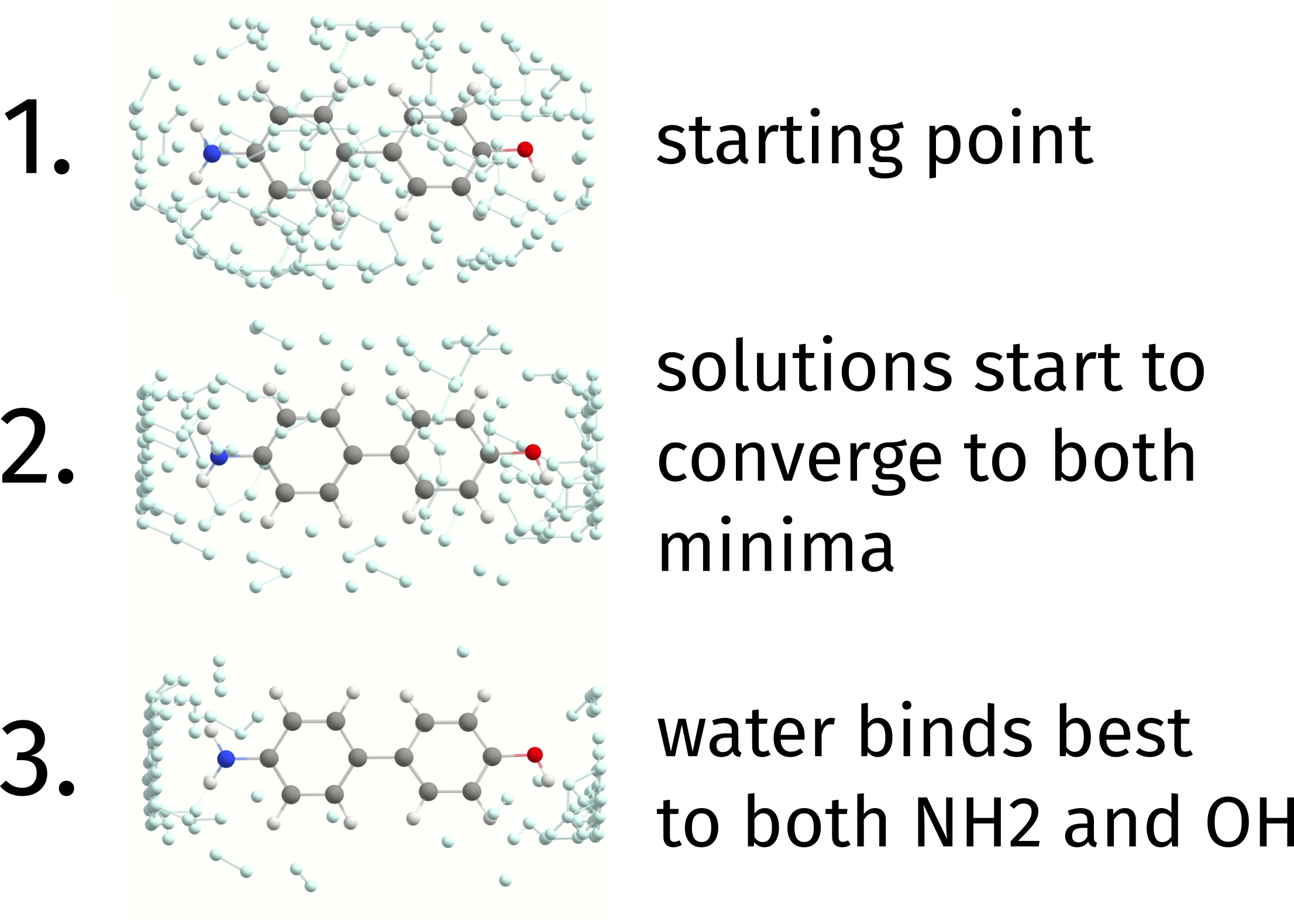
Fig. 7.60 The docking process of a water molecule on the substituted biphenyl.
Important
Right now the DOCKER can only be used together with the fast GFN-XTB methods, it will be generalized later. It is also not fully exploring the parallelization potential yet, and can be much faster for the next versions.
7.46.2. Looking Deeper into the Output
The details related to the grid and the swarm optimization can be found on the output, here is one example taken from the water dimer example from the earlier section:
Creating spatial grid
   Grid Max Dimension                5.50 Angs
   Angular Grid Step                 32.73 degrees
   Cartesian Grid Step               0.50 Angs
   Points per Dimension              11 points
Initializing workers
   Population Density                0.50 worker/Ang^2
   Population Size                   57
Evolving structures
   Minimization Algorithm            mutant particle swarm
   Min, Max Iterations               (3 , 10)
The Population Density here defines how many solutions will be placed on the initial grid around the HOST and can be controlled by %DOCKER POPDENSITY 0.50 END, while the population size is a direct consequence of that, unless specified by POPSIZE under %DOCKER.
Another important piece of information is the Min, Max Iterations, which define the minimum number of iterations before checking for convergence, and the maximum possible number of iterations. These can be changed by setting MINITER and MAXITER under the %DOCKER.
Then during the swarm search itself (here called the “evolution step”), the HOST and GUEST are partially optimized using the same criteria as from !SLOPPYOPT, and their energy at convergence is taken as a convergence criteria. The printing, still for the previous example, reads:
Note
All of the optimizations respect constraints and/or wall potentials given on the %GEOM block. The HOST can be easily frozen with %DOCKER FIXHOST TRUE END.
   Iter   Emin          avDE         stdDE            Time
          (Eh)       (kcal/mol)    (kcal/mol)        (min)
   -------------------------------------------------------

       1 -10.147462     2.756033     1.821981         0.03
       2 -10.147462     2.121389     1.610208         0.03
       3 -10.148583     2.313606     1.365227         0.03
       4 -10.148583     1.846998     1.188680         0.02
       5 -10.148583     1.587332     1.168207         0.02
No new minimum found after 3 (MinIter) steps.
Here we have the number of iterations, the energy of the best solution found during the process, the average energy difference from the lowest solutions and its standard deviation. The first number shows if the system is evolving towards a lower energy solutions and the later two give an idea of the “spread” of the energies found.
If no new minimum is found over MINITER iterations, the algorithm is considered to be converged and the best solutions are taken to the final optimization step.
7.46.3. The final steps
After the evolution step, a total of \(max(sqrt(PopSize),5)\) structures are taken from the set of solutions for a final full optimization. The output looks like:
Running final optimization
   Maximum number of structures      7
   Minimum energy difference         0.10 kcal/mol
   Maximum RMSD                      0.25 Angs
   Optimization strategy             regular
   Coordinate system                 redundant 2022
   Fixed host                        false
To avoid redundant solutions being optimized here, a check is made such that only structures with an energy difference of at least a Minimum energy difference and Maximum RMSD (obtained after an optimal rotation using the quaternion approach) are taken. The coordinate system might also be automatically set to Cartesian if the number of atoms is above 300 to speedup.
If some optimizations fail during the process, they will be flagged as optimization failed, as in the example below:
   Struc   Eopt       Interaction Energy       Time
           (Eh)               (kcal/mol)      (min)
   ------------------------------------------------

    1      -10.149006          -4.968378       0.01
    2      -10.149005          -4.967965       0.01
    3       optimization failed                0.01
    4      -10.149007          -4.968641       0.01
   (...)
That only means some of the solutions failed to fully optimize at the end, and on the printed file their energy is set to 1000 Eh to show the job was not completed. If you want to increase the number of iterations, or change the final convergence criteria, just change them using the %GEOM block as usual.
7.46.4. General Tips
In order to quick change the PES of the docking process, you can use
!DOCK(GFN2-XTB),!DOCK(GFN1-XTB),!DOCK(GFN0-XTB)or!DOCK(GFN-FF).For a quicker and less accurate docking the input
!QUICKDOCKis also available.There are four levels of “docking” procedure, from simple to more elaborate:
SCREENING,QUICK,NORMAL(default) andCOMPLETE, which can be given as%DOCK DOCKLEVEL COMPLETE END.To increase the final number of structures optimized in the end, just change
NOPTunder%DOCKER.If the guest topology is somehow changed during the docking process, that structure will be discarded. This can be turned off by setting
%DOCK CHECKGUESTTOPO FALSE END.
Important
By the time of the ORCA6 release, this algorithm was still not published. Publications are under preparation.
7.46.5. Complete Keyword List
!QUICKDOCK       # simple keyord to set DOCKLEVEL QUICK
!NORMALDOCK      # simple keyord to set DOCKLEVEL NORMAL
!COMPLETEDOCK    # simple keyord to set DOCKLEVEL COMPLETE

!DOCK(GFN-FF)    # simple keyord to set EVPES GFNFF
!DOCK(GFN0-XTB)  # simple keyord to set EVPES GFN0XTB
!DOCK(GFN1-XTB)  # simple keyord to set EVPES GFN1XTB
!DOCK(GFN2-XTB)  # simple keyord to set EVPES GFN2XTB

%DOCKER

   #
   # general options
   #

   GUEST           "filename.xyz" # an .xyz file (can be multistructure), from where
                                  # the guest(s) will be read. can contain different
                                  # charges and multiplicities for each guests on the
                                  # comment line. will only be read if exactly two
                                  # integer numbers are given, otherwise ignored.

   DOCKLEVEL       SCREENING  # defines a general strategy for docking.
                   QUICK      # will alter things like that population density
                   NORMAL     # and final number of optimized structrures.
                   COMPLETE   # default is NORMAL.

   PRINTLEVEL      LOW
                   NORMAL     # default
                   HIGH       # will print many extra files!

   NREPEATGUEST    1          # number of times to repeat the content of the "GUEST" file
   CUMULATIVE      TRUE       # add the contents of the "GUEST" file one on
                              # top of each other?
                              # default is FALSE, meaning each will be done independently.

   GUESTCHARGE     0          # can be used to defined a charge for the guest (default 0)
   GUESTMULT       3          # same for multiplicty (default 1)
                              # both can also be given via the comment line of the
                              # "filename.xyz", see above.

   RAMDOMSEED      TRUE       # whether to allow for the process to be trully random and
                              # will give different results everytime (default FALSE)

   FIXHOST         TRUE       # freeze coordinatef for the HOST during all steps?
                              # (default FALSE)

   CHECKGUESTTOPO  FALSE      # make sure that the topolgy of the GUEST is always kept
                              # (default TRUE)

   #
   # evolution step
   #

   MAXITER         10         # maximum number of iterations
   MINITER         3          # minimum number to check for convergence
                              # and minimum required of equal steps
                              # to signal convergence
   POPDENSITY      0.5        # the population density based on the HOST grid
   POPSIZE         150        # a fixed number for the swarm population size

   EVOPTLEVEL      NORMALOPT  # use default optimization criteria during the evolution step
                              # instead of the !SLOPPYOPT? more accurate, but slower.

   EVPES           GFNFF      # which PES to use **only** during the evolution step.
                   GFN0XTB    # can be different from the final optimization.
                   GFN1XTB
                   GFN2XTB
   #
   # final optimization
   #

   NOPT            10         # a fixed number of structures to be optimized
   NOOPT           FALSE      # do not optimize any structure at all? (default FALSE)