7.13. The Second Order Many Body Pertubation Theory Module (MP2)
Throughout this section, indices \(i,j,k,\dots\) refer to occupied orbitals in the reference determinant, \(a,b,c, \dots\) to virtual orbitals and \(p,q,r,\dots\) to general orbitals from either set while \(\mu ,\nu ,\kappa ,\tau , \dots\) refer to basis functions.
7.13.1. Standard MP2
The standard (or full accuracy) MP2 module has two different branches. One branch is used for energy calculations, the other for gradient calculations.
For standard MP2 energies, the program performs two half-transformations and the half-transformed integrals are stored on disk in compressed form. This appears to be the most efficient approach that can also be used for medium sized molecules.The module should parallelize acceptably well as long as I/O is not limiting.
For standard MP2 gradients, the program performs four quarter
transformations that are ordered by occupied orbitals. Here, the program
massively benefits from large core memory (%maxcore) since this
minimizes the number of batches that are to be done. I/O demands are
minimal in this approach.
In “memory mode” (Q1Opt>0) basically the program treats batches of occupied orbitals at the same time. Thus, there must be at least enough memory to treat a single occupied MO at each pass. Otherwise the MP2 module will fail. Thus, potentially, MP2 calculations on large molecules take significant memory and may be most efficiently done through the RI approximation.
Alternatively, in the “disk based mode” (Q1Opt\(=\)-1) the program
performs a half transformation of the exchange integrals and stores the
transformed integrals on disk. A bin-sort then leads to the AO operator
\(K^{ij} \left(\mu ,\nu\right)=\left(i\mu|j\nu \right)\) in (11|22)
integral notation. These
integrals are then used to make the final K\(^{ij}\)(a,b) (a,b\(=\)virtual
MOs) and the EMP2 pair energy contributions. In many cases, and in
particular for larger molecules, this algorithm is much more efficient
than the memory based algorithm. It depends, however, much more heavily
on the I/O system of the computer that you use. It is important, that
the program uses the flags CFLOAT, UCFLOAT, CDOUBLE or UCDOUBLE in
order to store the unsorted and sorted AO exchange integrals. Which flag
is used will influence the performance of the program and to some extent
the accuracy of the result (float based single precision results are
usually very slightly less accurate; \(\mu\)Eh-range deviations from the
double precision result[1]). Finally, gradients are presently only
available for the memory based algorithm since in this case a much
larger set of integrals is required.
The ! MP2 command does the following: (a) it changes the Method to
HFGTO and (b) it sets the flag DoMP2 to true. The program will
then first carry out a Hartree-Fock SCF calculation and then estimate
the correlation energy by MP2 theory. RHF, UHF and high-spin ROHF
reference wavefunctions are permissible and the type of MP2 calculation
to be carried out (for high-spin ROHF the gradients are not available)
is automatically chosen based on the value of HFTyp. If the SCF is
carried out conventionally, the MP2 calculation will also be done in a
conventional scheme unless the user forces the calculation to be direct.
For SCFMode \(=\)Direct the MP2 energy evaluation will be fully in the
integral direct mode.
The following variables can be adjusted in the block for conventional MP2 calculations:
%mp2
  EMin       -1.5       # orbital energy cutoff that defines the
                        # frozen core in Eh
  EMax        1.0e3     # orbital energy cutoff that defines the
                        # neglected virtual orbitals in Eh
  EWin        EMin,EMax # the same, but accessed as array
                        # (respects settings in %method block!)
  MaxCore     256       # maximum amount of memory (in MB) to be
                        # used for integral buffering
  ForceDirect false     # Force the calculation to be integral
                        # direct
  RI          false     # use the RI approximation
  F12         false     # apply F12 correction
  Q1Opt                 # For non-RI calculations a flag how to perform
                        # the first quarter transformation
                        #  1 - use double precision buffers
                        #      (default for gradient runs)
                        #  2 - use single precision buffers. This reduces
                        #      the memory usage in the bottleneck step by
                        #      a factor of two. If several passes are re-
                        #      quired, the number of passes is reduced by
                        #      a factor of two.
                        # -1 - Use a disk based algorithm. This respects
                        #      the flags UCFLOAT,CFLOAT,UCDOUBLE and
                        #      CDOUBLE. (but BE CAREFUL with FLOAT)
                        #      (default for energy runs)
  PrintLevel  2         # How much output to produce. PrintLevel 3 produces
                        # also pair correlation energies and other info.
  DoSCS       false     # use spin-component scaling
  Ps          1.2       # scaling factor for ab pairs
  Pt          0.333     # scaling factor for aa and bb pairs
  Density     none      # no density construction
              unrelaxed # only "unrelaxed densities"
              relaxed   # full relaxed densities
  NatOrbs     false     # calculate natural orbitals
7.13.2. RI-MP2
The RI-MP2 module is of a straightforward nature. The program first transforms the three-index integrals \((ia| \tilde{P})\), where “\(i\)” is a occupied, “\(a\)” is a virtual MO and “\(\tilde{P}\)” is an auxiliary basis function that is orthogonalized against the Coulomb metric. These integrals are stored on disk, which is not critical, even if the basis has several thousand functions. The integral transformation is parallelized and has no specifically large core memory requirements.
In the next step, the integrals are read ordered with respect to the occupied labels and the exchange operators \(K^{ij}(a,b) = (ia| jb) = \sum_{\tilde{P} }^{\text{NAux} } (ia | \tilde{P})(\tilde{P} | jb)\) are formed in the rate limiting O(N\(^{5})\) step. This step is done with high efficiency by a large matrix multiplication and parallelizes well. From the exchange operators, the MP2 amplitudes and the MP2 energy is formed. The program mildly benefits from large core memory (%maxcore) as this minimizes the number of batches and hence reads through the integral list.
The RI-MP2 gradient is also available. Here, all necessary intermediates are made on the fly.
In the RI approximation, one introduces an auxiliary fitting basis \(\eta_{P} \left({ \mathrm{\mathbf{r} }} \right)\) and then approximates the two-electron integrals in the Coulomb metric as:
where \(V_{PQ} =\left({ P\vert Q} \right)\) is a two-index electron-electron repulsion integral. As first discussed by Weigend and Häser, the closed-shell case RI-MP2 gradient takes the form:
The F-matrix derivative terms are precisely handled as in the non-RI case and need not be discussed any further. \(\Gamma_{ia}^{P}\) is a three-index two-particle “density”:
Which is partially transformed to the AO basis by:
The two-index analogue is given by:
The RI contribution to the Lagrangian is particularly convenient to calculate:
In a similar way, the remaining contributions to the energy weighted density matrix can be obtained efficiently. Note, however, that the response operator and solution of the CP-SCF equations still proceed via traditional four- index integrals since the SCF operator was built in this way. Thus, while the derivatives of the three-index integrals are readily and efficiently calculated, one still has the separable contribution to the gradient, which requires the derivatives of the four-index integrals.
The RI-MP2 energy and gradient calculations can be drastically accelerated by employing the RIJCOSX or the RIJDX approximation.
7.13.3. “Double-Hybrid” Density Functional Theory
A slightly more general form is met in the double-hybrid DFT gradient. The theory is briefly described below.
The energy expression for perturbatively and gradient corrected hybrid functionals as proposed by Grimme is:
Here \(V_{NN}\) is the nuclear repulsion energy and \(h_{\mu \nu }\) is a matrix element of the usual one-electron operator which contains the kinetic energy and electron-nuclear attraction terms (\(\left\langle {\mathrm{\mathbf{ab} }} \right\rangle\) denotes the trace of the matrix product \(\mathrm{\mathbf{ab} })\). As usual, the molecular spin-orbitals are expanded in atom centered basis functions (\(\sigma =\alpha ,\beta )\):
with MO coefficients \(c_{\mu p}^{\sigma }\). The total density is given by (real orbitals are assumed throughout):
Where \(\mathrm{\mathbf{P} }=\mathrm{\mathbf{P} }^{\alpha }+\mathrm{\mathbf{P} }^{\beta }\) and \(P_{\mu \nu }^{\sigma } =\sum_{i_{\sigma } } { c_{\mu i}^{\sigma } c_{\nu i}^{\sigma } }\).
The second term of (7.56) represents the Coulombic self-repulsion. The third term represents the contribution of the Hartree-Fock exchange with the two-electron integrals being defined as:
The mixing parameter \(a_{x}\) controls the fraction of Hartree-Fock exchange and is of a semi-empirical nature. The exchange correlation contribution may be written as:
Here, \(E_{\text{X} }^{\text{GGA} } \left[{ \rho_{\alpha } ,\rho_{\beta } } \right]\) is the exchange part of the XC- functional in question and \(E_{\text{C} }^{\text{GGA} } \left[{ \rho_{\alpha } ,\rho_{\beta } } \right]\) is the correlation part. The parameter \(b\) controls the mixing of DFT correlation into the total energy and the parameter \(c_{\text{DF} }\) is a global scaling factor that allows one to proceed from Hartree-Fock theory (\(a_{\text{X} } =1\), \(c_{\text{DF} } =0\), \(c_{\text{PT} } =0)\) to MP2 theory (\(a_{\text{X} } =1\), \(c_{\text{DF} } =0\), \(c_{\text{PT} } =1\)) to pure DFT (\(a_{\text{X} } =1\), \(c_{\text{DF} } =0\), \(c_{\text{PT} } =1\)) to hybrid DFT (\(0 < a_{\text{X} } <1\), \(c_{\text{DF} } =1\), \(c_{\text{PT} } =0)\) and finally to the general perturbatively corrected methods discussed in this work (\(0<a_{\text{X} } <1\), \(c_{\text{DF} } =1\), \(0<c_{\text{PT} } <1\)). As discussed in detail by Grimme, the B2- PLYP functional uses the Lee-Yang-Parr (LYP) functional as correlation part, the Becke 1988 (B88) functional as GGA exchange part and the optimum choice of the semi-empirical parameters was determined to be \(a_{\text{X} } =0.53\), \(c_{\text{PT} } =0.27\), \(c_{\text{DF} } =1\), \(b=1-c_{\text{PT} }\). For convenience, we will suppress the explicit reference to the parameters \(a_{\text{X} }\) and \(b\) in the XC part and rewrite the gradient corrected XC energy as:
with the gradient invariants \(\gamma^{\sigma{ \sigma }'}=\vec{{\nabla } }\rho^{\sigma }\vec{{\nabla } } \rho^{{\sigma }'}\). The final term in eq (48) represents the scaled second order perturbation energy:
The PT2 amplitudes have been collected in matrices \(\mathrm{\mathbf{t} }^{i_{\sigma } j_{{\sigma }'} }\) with elements:
Where the orbitals were assumed to be canonical with orbital energies \(\varepsilon_{p}^{\sigma }\). The exchange operator matrices are \(K_{a_{\sigma } b_{{\sigma }'} }^{i_{\sigma } j_{{\sigma }'} } =\left({ i_{\sigma } a_{\sigma } \vert j_{{\sigma }'} b_{{\sigma }'} } \right)\) and the anti-symmetrized exchange integrals are defined as \(\bar{{K} }_{a_{\sigma } b_{{\sigma }'} }^{i_{\sigma } j_{{\sigma }'} } =\left({ i_{\sigma } a_{\sigma } \vert j_{{\sigma }'} b_{{\sigma }'} } \right)-\delta_{\sigma{ \sigma }'} \left({ i_{\sigma } b_{\sigma } \vert _{\sigma } a_{\sigma } } \right)\).
The orbitals satisfy the SCF equations with the matrix element of the SCF operator given by:
The matrix elements of the XC–potential for a gradient corrected functional are: [840]
The energy in equation (7.56) depends on the MO-coefficients, the PT2-amplitudes and through \(V_{NN}\), \(V_{eN}\) (in \(h)\) and the basis functions also explicitly on the molecular geometry. Unfortunately, the energy is only stationary with respect to the PT2 amplitudes since they can be considered as having been optimized through the minimization of the Hylleraas functional:
The unrelaxed PT2 difference density is defined as:
With analogous expressions for the spin-down unrelaxed difference densities. Minimization of this functional with respect to the amplitudes yields the second order perturbation energy. The derivative of the SCF part of equation (7.56) with respect to a parameter “\(x\)” is straightforward and well known. It yields:
Superscript “\(x\)” refers to the derivative with respect to some perturbation “\(x\)” while a superscript in parentheses indicates that only the derivative of the basis functions with respect to “\(x\)” is to be taken. For example:
In equation (7.69), S is the overlap matrix and W \(^{\text{SCF} }\) the energy weighted density:
At this point, the effective two-particle density matrix is fully separable and reads:
The derivative of the PT2 part is considerably more complex, since \(E_{\text{PT2} }\) is not stationary with respect to changes in the molecular orbitals. This necessitates the solution of the coupled-perturbed SCF (CP-SCF) equations. We follow the standard practice and expand the perturbed orbitals in terms of the unperturbed ones as:
The occupied-occupied and virtual-virtual blocks of U are fixed, as usual, through the derivative of the orthonormality constraints:
Where \(S_{pq}^{\sigma \left( x \right)} =\sum\nolimits_{\mu \nu } { c_{\mu p}^{\sigma } c_{\nu q}^{\sigma } S_{\mu \nu }^{\left( x \right)} }\). The remaining virtual-occupied block of U \(^{x}\) must be determined through the solution of the CP-SCF equations. However, as shown by Handy and Schaefer, this step is unnecessary and only a single set of CP-SCF equations (Z-vector equations) needs to be solved. To this end, one defines the Lagrangian:
An analogous equation holds for \(L_{ai}^{\beta }\). The matrix elements of the response operator \(R^{\alpha } \left({ \mathrm{\mathbf{D}'} } \right)\) are best evaluated in the AO basis and then transformed into the MO basis. The AO basis matrix elements are given by:
where
The \(\zeta\)-gradient-parameters are evaluated as a mixture of PT2 difference densities and SCF densities. For example:
With
Having defined the Lagrangian, the following CP-SCF equations need to be solved for the elements of the “Z- vector”:
The solution defines the occupied-virtual block of the relaxed difference density, which is given by:
For convenience, \(\mathrm{\mathbf{D} }^{\sigma }\) is symmetrized since it will only be contracted with symmetric matrices afterwards. After having solved the Z-vector equations, all parts of the energy weighted difference density matrix can be readily calculated:
Once more, analogous equations hold for the spin-down case. With the relaxed difference density and energy weighted density matrices in hand, one can finally proceed to evaluate the gradient of the PT2 part as \((\mathrm{\mathbf{W} } ^{\text{PT2} }=\mathrm{\mathbf{W} }^{\alpha ;\text{PT2} }+\mathrm{\mathbf{W} }^{\beta ;\text{PT2} })\):
The final derivative of eq. (7.56) is of course the sum \(E_{SCF}^{x} +c_{PT} E_{\text{PT2} }^{x}\). Both derivatives should be evaluated simultaneously in the interest of computational efficiency.
Note that the exchange-correlation contributions to the gradient take a somewhat more involved form than might have been anticipated. In fact, from looking at the SCF XC-gradient (eq. (7.69)) it could have been speculated that the PT2 part of the gradient is of the same form but with \(\rho_{\mathrm{\mathbf{P} }}^{\sigma \left( x \right)}\) being replaced by \(\hat{{H} }\), the relaxed PT2 difference density. This is, however, not the case. The underlying reason for the added complexity apparent in equation (7.89) is that the XC contributions to the PT2 gradient arise from the contraction of the relaxed PT2 difference density with the derivative of the SCF operator. Since the SCF operator already contains the first derivative of the XC potential and the PT2 energy is not stationary with respect to changes in the SCF density, a response type term arises which requires the evaluation of the second functional derivative of the XC-functional. Finally, as is well known from MP2 gradient theory, the effective two- particle density matrix contains a separable and a non-separable part:
Thus, the non-separable part is merely the back-transformation of the amplitudes from the MO to the AO basis. It is, however, important to symmetrize the two-particle density matrix in order to be able to exploit the full permutational symmetry of the AO derivative integrals.
7.13.4. Orbital Optimized MP2
The MP2 energy can be regarded as being stationary with respect to the MP2 amplitudes, since they can be considered as having been optimized through the minimization of the Hylleraas functional:
\(\hat{{H} }\) is the 0\(^{th}\) order Hamiltonian as proposed by Møller and Plesset, \(\Psi_{0}\) is the reference determinant, \(\Psi_{1}\) is the first-order wave function and \(E_{0} =E_{\text{HF} } =\left\langle\Psi_{\text{HF} } \right|\hat{{H} }\left| \Psi_{\text{HF} }\right\rangle\) is the reference energy. The quantities \(\mathbf{t}\) collectively denote the MP2 amplitudes.
The fundamental idea of the OO-MP2 method is to not only minimize the MP2 energy with respect to the MP2 amplitudes, but to minimize the total energy additionally with respect to changes in the orbitals. Since the MP2 energy is not variational with respect to the MO coefficients, no orbital relaxation due to the correlation field is taken into account. If the reference determinant is poor, the low-order perturbative correction then becomes unreliable. This may be alleviated to a large extent by choosing better orbitals in the reference determinant. Numerical evidence for the correctness of this assumption will be presented below.
In order to allow for orbital relaxation, the Hylleraas functional can be regarded as a functional of the wavefunction amplitudes \(\mathbf{t}\) and the orbital rotation parameters \(\mathbf{R}\) that will be defined below. Through a suitable parameterization it becomes unnecessary to ensure orbital orthonormality through Lagrange multipliers. The functional that we minimize reads:
\(\Psi_{0}\) is the reference determinant. However, it does no longer correspond to the Hartree-Fock (HF) determinant. Hence, the reference energy \(E_{0} \left[{ \mathbf{R} } \right]=\left\langle { \Psi_{0} \left[{ \mathbf{R} } \right]} \right|\hat{{H} }\left|\Psi_{0} \left[{ \mathbf{R} } \right] \right\rangle\) also changes during the variational process and is no longer stationary with respect to the HF MO coefficients. Obviously, \(E_{0} \left[{ \mathbf{R} } \right]\geqslant E_{\text{HF} }\) since the HF determinant is, by construction, the single determinant with the lowest expectation value of the full Hamiltonian.
The reference energy is given as:
The first-order wave function excluding single excitations is:
A conceptually important point is that Brillouin’s theorem [419] is no longer obeyed since the Fock matrix will contain off-diagonal blocks. Under these circumstances the first-order wavefunction would contain contributions from single excitations. Since the orbital optimization brings in all important effects of the singles we prefer to leave them out of the treatment. Any attempt to the contrary will destroy the convergence properties. We have nevertheless contemplated to include the single excitations perturbatively:
The perturbative nature of this correction would destroy the stationary nature of the total energy and is hence not desirable. Furthermore, results with inclusion of single excitation contributions represent no improvement to the results reported below. They will therefore not be documented below and henceforth be omitted from the OO-MP2 method by default.
The explicit form of the orbital-optimized MP2 Hylleraas functional employing the RI approximation (OO-RI-MP2) becomes:
with:
Here, \(\left\{\psi \right\}\) is the set of orthonormal molecular orbitals and \(\left\{\eta \right\}\) denotes the auxiliary basis set. \(F_{pq}\) denotes a Fock matrix element:
and it is insisted that the orbitals diagonalize the occupied and virtual subspaces, respectively:
The MP2 like density blocks are,
where the MP2 amplitudes in the case of a block diagonal Fock matrix are obtained through the condition\(\frac{\partial L_{\infty} }{\partial t_{ab}^{ij} }=0\):
The orbital changes are parameterized by an anti-Hermitian matrix \(\mathbf{R}\) and an exponential Ansatz,
The orbitals changes to second order are,
Through this Ansatz it is ensured that the orbitals remain orthonormal and no Lagrangian multipliers need to be introduced. The first-order expansion of the Fock operator due to the orbital rotations are:
The first-order energy change becomes \(\left({ h_{pq} \equiv \left\langle p \right|\hat{{h} }\left| q \right\rangle,g_{pqrs} \equiv \left\langle { pq} || rs \right\rangle} \right)\):
The condition for the energy functional to be stationary with respect to the orbital rotations \(\left({ \frac{\partial L_{\infty} \left[{ \mathbf{t,R} } \right]}{\partial R_{ai} }=0} \right)\), yields the expression for the orbital gradient and hence the expression for the OO-RI-MP2 Lagrangian.
The goal of the orbital optimization process is to bring this gradient to zero. There are obviously many ways to achieve this. In our experience, the following simple procedure is essentially satisfactory. We first build a matrix \(\mathbf{B}\) in the current MO basis with the following structure:
where \(\Delta\) is a level shift parameter. The occupied/occupied and virtual/virtual blocks of this matrix are arbitrary but their definition has a bearing on the convergence properties of the method. The orbital energies of the block diagonalized Fock matrix appear to be a logical choice. If the gradient is zero, the B-matrix is diagonal. Hence one obtains an improved set of orbitals by diagonalizing B.
In order to accelerate convergence a standard DIIS scheme is used. [451, 576] However, in order to carry out the DIIS extrapolation of the B-matrix it is essential that a common basis is used that does not change from iteration to iteration. Since the B-matrix itself is defined in the molecular orbitals of the current iteration we choose as a common set of orthonormal orbitals the MOs of the HF calculation. The extrapolation is carried out in this basis and the extrapolated B-matrix is transformed back to the current set of MOs prior to diagonalization. Obviously, the same strategy can be used for orbital optimization in any method for which an orbital gradient is available.
For well behaved cases this simple scheme converges in 5-10 iterations. Transition metals and more complicated molecules may require up to 20 iterations and level shifting in order to achieve convergence.
Upon convergence the sum of the matrix \(\mathbf{D}\) and the density of the reference determinant \(P_{\mu \nu } =\sum_i { c_{\mu i} c_{\nu i} }\) form the true one-particle density matrix of the OO-MP2 approach that can be used for property or gradient calculations.
7.13.5. Regularized MP2 and RI-MP2
Regularized MP2 is a variant of second-order Moller-Plesset theory (MP2) introduced by J. Shee, M. Loipersberger, A. Rettig, J. Lee, and M. Head-Gordon [791] that aims to improve its accuracy for systems with \(\pi\)-driven dispersion interactions and dative bonds in transition metal complexes. The approach achieves this by introducing a single-parameter, energy-gap dependent regularization that dampens overestimated pairwise additive contributions, thus renormalizing first-order amplitudes to empirically mimic higher-order correlations.
For this, the standard MP2 energy and thus the standard algorithms are modified. For the \(\sigma\) \(\text{(}p=1\text{)}\) and \(\sigma^2\) \(\text{(}p=2\text{)}\) regularization, the energy is modified according to
which corresponds to regularizing the first-order amplitudes. For the \(\kappa\) regularization, the MP2 energy is modified according to
which corresponds to regularizing the first-order amplitudes and the exchange integrals.
Regularized MP2 is available for standard MP2 in “memory mode” (Q1Opt\(>\)0) and RI-MP2 (RIJDX, RIJCOSX, RIJK).
The usage of regularized MP2 is controlled by the DoRegMP2 keyword, the type of regularization can be specified by setting the RegMP2Type parameter to 0 for \(\kappa\), 1 for \(\sigma\), or 2 for \(\sigma^2\). The value of the regularizers can be specified by RegMP2Kappa and RegMP2Sigma respectively.
%mp2
    DoRegMP2     true   # required
    RegMP2Type   0      # kappa regularizer
                 1      # sigma regularizer
                 2      # sigma-sqaured regularizer
    RegMP2Kappa  1.1    # kappa value
    RegMP2Sigma  0.5    # sigma value
end
It is important to note that only single point energies are available and tested for regularized MP2. Density, Gradient, and Hessian calculations are not yet supported.
7.13.6. RIJCOSX-RI-MP2 Gradients
Additional grids are introduced for the RIJCOSX-MP2 gradient. They have sensible default settings and therefore do not usually require any intervention from the user. However, a number of expert options are available, as described below.
The COSX terms in the Z-vector equations are calculated on a grid,
controlled by the keywords Z_GridX and Z_IntAccX, as discussed in
sections Changing TD-DFT, CP-SCF and Hessian grids and
CP-SCF Options. For example, the DefGrid3 CP-SCF COSX
grid can be requested as:
%method
  Z_GridX   2     # Lebedev 110-point grid
  Z_IntAccX 3.067 # radial integration accuracy
end
The grid used for evaluation of the response operator on the right-hand
side of the Z-vector equations (see for example
eqs (7.77) and
(7.78)) can be independently selected using the
keyword Z_GridX_RHS. Note that starting with ORCA 5, the usage is
different to Z_GridX - the choice is between one of the three grids
used during the RIJCOSX SCF procedure: a small grid for the initial
iterations, a medium grid for the final iterations (default in ORCA 5),
and a large grid to evaluate the energy more accurately after the
iterations have converged.
%method
  Z_GridX_RHS 1  # small SCF grid
              2  # medium SCF grid (default)
              3  # large SCF grid
end
Yet another grid is used to evaluate basis functions derivatives.
Appropriate parameters are chosen through ! DefGridn (in addition to
the three SCF grids), but one can override this by setting the angular
(GridX) and radial (IntAccX) grids explicitly through:
%mp2 GridX    4       # default 4: angular Lebedev grid 302
     IntAccX  4.871   # radial grid
end
7.13.7. MP2 and RI-MP2 Second Derivatives
Analytical second-order properties with the MP2, RI-MP2 and
double-hybrid DFT methods are available in ORCA for calculations without
frozen core orbitals. The most expensive term in the second derivative calculations is the four-external contribution which can be evaluated either via an AO direct (default) or a semi-numerical Chain-of-Spheres approach. In case
that the latter approach is chosen, appropriate grid parameters are
defined through the ! DefGridn settings. However, a more fine-grained
specification is available to expert users as follows:
%mp2 KCOpt _AOBLAS          # (default) AO direct with BLAS routines
           _COSX            # semi-numerical evaluation using the COSX method
     KC_GridX    2          # default 2: angular Lebedev grid 110
     KC_IntAccX  4.020      # radial grid
end
Alternatively, all the grid settings can be defined in the %method
block, as discussed in
section SCF grid keyword list. The first three entries
define the three SCF grids, the fourth entry the MP2 grid for basis
function derivatives (refer to
section RIJCOSX-RI-MP2 Gradients) and the fifth entry the
grid for the four-external contribution.
%method
   IntAccX     Acc1,  Acc2,  Acc3,  Acc4,   Acc5
   GridX       Ang1,  Ang2,  Ang3,  Ang4,   Ang5
end
7.13.8. RI-MP2 and Double-Hybrid DFT Response Properties
Starting from ORCA 5, both the electric (for the dipole polarizability) and the magnetic (for NMR shielding and the EPR g-tensor) field response as well as the nucleus-orbit response (hyperfine couplings \(A_\text{orb}\) term) for RI-MP2 (and double-hybrid functionals) is handled by a different implementation of the RI-MP2 second derivatives than that used for geometric Hessian calculations (MP2 and RI-MP2 Second Derivatives). This code is more efficient, uses the RI approximation throughout (including the four-external contribution) and supports frozen core orbitals. The implementation is described in detail in refs [829, 850]. Consider the following input for a GIAO-RI-MP2 NMR shielding calculation:
! RIJK RI-MP2 def2-SVP def2/JK def2-SVP/C TightSCF NMR NoFrozenCore
%mp2
  Density         relaxed # required
  UsePertCanOrbs  true    # Whether to use perturbed canonical orbitals for
                          # the internal block of the perturbed Fock matrix
  PertCan_EThresh 1e-6    # Energy threshold for special treatment of
                          # degenerate orbital pairs
  PertCan_UThresh 10      # Coefficient threshold for special treatment of
                          # strongly interacting orbital pairs
  FCut            1e-5    # Threshold for internal perturbed Fock elements
  RespStoreT      true    # Whether to precalculate and store all necessary
                          # unperturbed amplitudes on disk
  RespDijConv     false   # Whether to store intermediates required for the
                          # internal block of the response density on disk
end
* int 0 1
O 0 0 0 0      0      0
H 1 0 0 1.1056 0      0
H 1 2 0 1.1056 109.62 0
*
By default perturbed canonical orbitals are used for the occupied block, i.e., the internal orbital rotation coefficients are chosen as
which results in \(F^{\mathbf B}_{ij}=0\), thereby eliminating its contribution to the perturbed amplitudes:
If \(| \epsilon_j - \epsilon_i |<\) PertCan_EThresh or \(|U_{ij}^B| > \) PertCan_UThresh, then
\(U^{\mathbf B}_{ij}\) is chosen using the standard formula
And the relevant contributions to
eq (7.112) are added, unless
\(\left|F^{\mathbf B}_{ij}\right|< \) FCut. The required amplitudes
\(\mathbf T^{ik}\) and \(\mathbf T^{kj}\) (all amplitudes, in case
UsePertCanOrbs = false) are stored on disk if
RespStoreT = true or recalculated as needed otherwise.
The latter option is significantly slower and not recommended unless
disk space is an issue. Similarly, in the case of insufficient RAM, the
option RespDijConv = true tells ORCA to store all
amplitudes in the batch (required to calculate \(D_{ij}^\mathbf B\)) on
disk, rather than keep them in memory. The 3-index 2-particle densities,
needed for the right-hand side of the Z-vector equations, are always stored on disk.
Note also that in this implementation the RIJCOSX Fock-response terms
are calculated with one of the SCF grids, chosen with Z_GridX_RHS (see
section CP-SCF Options).
7.13.9. Local MP2
In analogy to the domain-based local pair natural orbital coupled-cluster methods, there is also a local linear scaling version of MP2 (DLPNO-MP2) implemented in ORCA. Its default thresholds are chosen to reproduce about 99.9% of the total RI-MP2 correlation energy, resulting in an accuracy of a fraction of \(1\,\text{kcal/mol}\) for energy differences. The theory has been described in the literature.[654, 685]
Further information of local correlation methods in ORCA can be found in section Local correlation. The local MP2 method becomes truly beneficial for very large molecules and can be used to compute energies of systems containing several hundred atoms. Fig. 7.3 shows the scaling behavior for linear alkane chains. Note that this represents an idealized situation. For three-dimensional molecules the crossover with canonical RI-MP2 is going to occur at a later point.
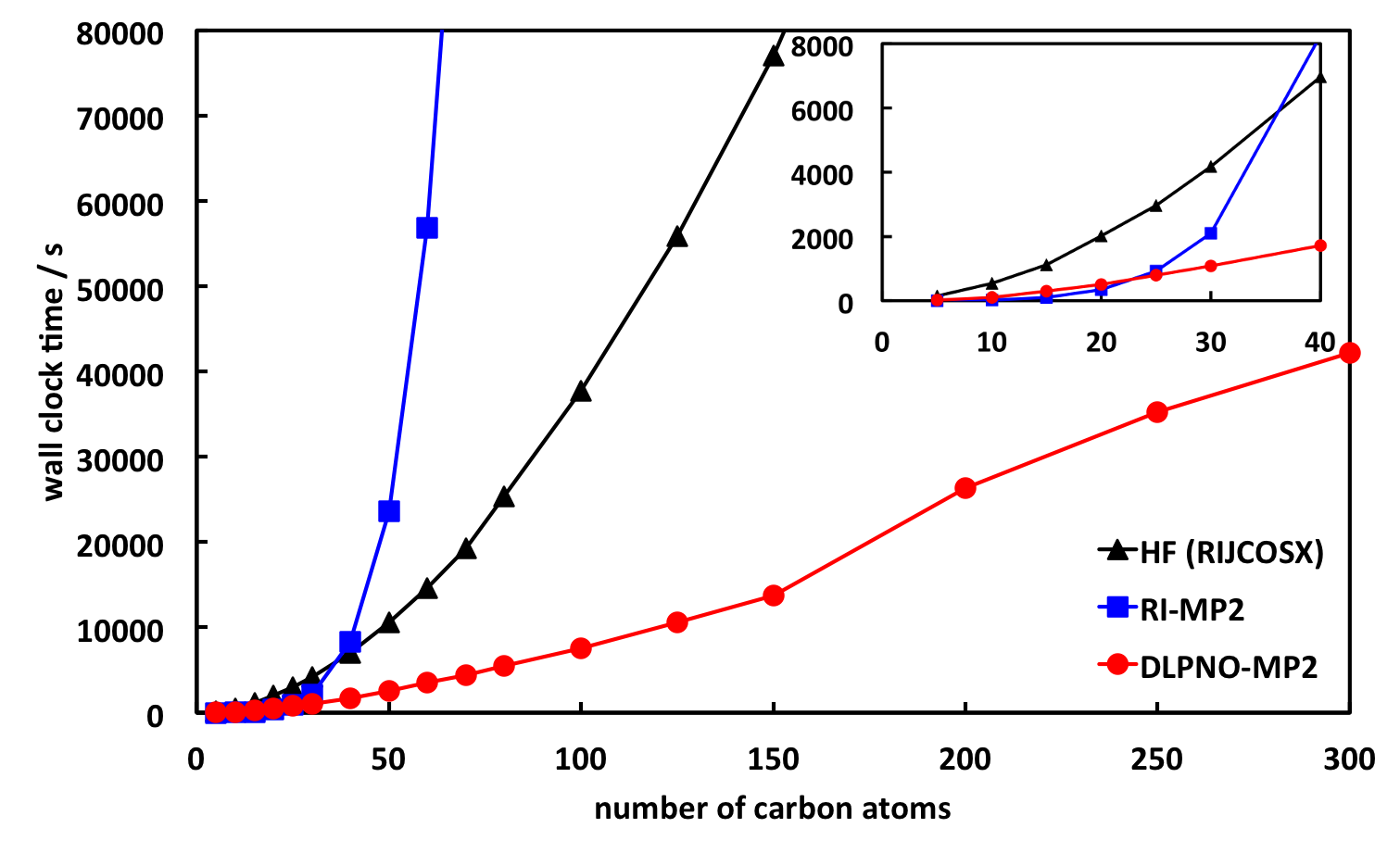
Fig. 7.3 Scaling of the DLPNO-MP2 method with default thresholds for linear alkane chains in def2-TZVP basis. Shown are also the times for the corresponding Hartree-Fock calculations with RIJCOSX and for RI-MP2.
In the following, the most important design principles of the RHF-DLPNO-MP2 are pointed out.
Unlike in the 2013 version of the DLPNO methodology, domains are selected by means of the differential overlap \(\sqrt{\int i^2(\mathbf{r}) \tilde\mu'^2 (\mathbf{r}) d\mathbf{r} }\) between localized MOs \(i\) and projected atomic orbitals (PAOs) \(\tilde\mu'\) which are normalized to unity. The default value for the corresponding cutoff is \(T_\text{CutDO}=10^{-2}\).
MP2 amplitudes for each pair of localized orbitals \(ij\) are expressed in a basis of pair natural orbitals (PNOs) \(\tilde a_{ij}\). PNOs are obtained from diagonalization of an approximate, “semicanonical” MP2 pair density \(\mathbf{D}^{ij}\). Only PNOs with an occupation number \(>T_\text{CutPNO}\) are retained, with a default value of \(T_\text{CutPNO} = 10^{-8}\) for DLPNO-MP2. The pair density is given by:
\[\begin{split}\mathbf{D}^{ij} = \mathbf{T}^{ij\dagger} \tilde{\mathbf{T} }^{ij} + \mathbf{T}^{ij} \tilde{\mathbf{T} }^{ij\dagger} \quad\text{where}\quad \begin{matrix}T^{ij}_{\tilde\mu\tilde\nu} = -\dfrac{\left(i\tilde\mu \middle| j \tilde\nu\right)}{\varepsilon_{\tilde\mu} + \varepsilon_{\tilde\nu} - F_{ii} - F_{jj} } \\ \tilde{\mathbf{T} }^{ij} = \left(1+\delta_{ij}\right)^{-1} \left( 4\mathbf{T}^{ij} - 2\mathbf{T}^{ij\dagger}\right)\end{matrix}\end{split}\]Since the occupied block of the Fock matrix is not diagonal in the basis of localized orbitals, the MP2 amplitudes \(\mathbf{T}^{ij}\) are obtained by solving the following set of residual equations iteratively (where subscripts of PNOs have been dropped):
\[R^{ij}_{\tilde a\tilde b} = \left(i \tilde a \middle| j \tilde b\right) + \left( \varepsilon_{\tilde a} + \varepsilon_{\tilde b} - F_{ii} - F_{jj} \right) T^{ij}_{\tilde a\tilde b} - \sum_{k\neq i} \sum_{\tilde c\tilde d} F_{ik} S^{ij, kj}_{\tilde a\tilde c} T^{kj}_{\tilde c \tilde d} S^{kj, ij}_{\tilde d\tilde b} - \sum_{k\neq j} \sum_{\tilde c\tilde d} F_{kj} S^{ij, ik}_{\tilde a\tilde c} T^{ik}_{\tilde c \tilde d} S^{ik, ij}_{\tilde d\tilde b} = 0\]The largest part of the error relative to canonical RI-MP2 is controlled by the domain (
TCutDO) and PNO (TCutPNO) thresholds, which should be adequate for most applications. If increased accuracy is needed (e.g. for studying weak interactions), tighter truncation criteria can be invoked by means of the! TightPNOkeyword. Conversely, a less accurate but faster calculation can be performed with the! LoosePNOkeyword. For more details refer to table Table 7.16.Fitting domains are determined by means of orbital Mulliken populations with a threshold \(T_\text{CutMKN} =10^{-3}\). This threshold results in an error contribution that is typically about an order of magnitude smaller than the overall total energy deviation from RI-MP2.
Prior to performing the local MP2 calculation, pairs of localized molecular orbitals \(ij\) are prescreened using an MP2 energy estimate with a dipole approximation, and the differential overlap integral between orbitals \(i\) and \(j\). This procedure has been chosen conservatively and leads to minimal errors.
Residual evaluation can be accelerated significantly by neglecting terms with associated Fock matrix elements \(F_{ik}\) and \(F_{kj}\) below \(F_\text{Cut}=10^{-5}\). Errors resulting from this approximation are typically below \(1\,\mu\text{E}_\text{h}\) and thus negligible.
Sparsity of the MO and PAO coefficient matrices in atomic orbital basis is exploited to accelerate integral transformations for large systems. Truncation of the coefficients is controlled by a parameter \(T_\text{CutC}\). Neglect of these coefficients has to be performed very carefully in order to avoid uncontrollable errors. The threshold has been chosen so as to make the errors essentially vanish.
By default, core orbitals are frozen in the MP2 module. However, if core orbitals are subject to an MP2 treatment, it is necessary to use a tighter PNO cutoff for pairs involving at least one core orbital. For this purpose core orbitals and valence orbitals are localized separately. The cutoff for pairs involving core orbitals is given by \(T_\text{CutPNO} \times T_\text{ScalePNO\_Core}\), where \(T_\text{ScalePNO\_Core}=10^{-2}\) by default. For more details refer to section Including (semi)core orbitals in the correlation treatment.
The UHF-DLPNO-MP2 implementation differs somewhat from the RHF case, particularly regarding construction of PNOs, as described below.
A separate set of PAOs \(\tilde\mu'_\alpha\) and \(\tilde\mu'_\beta\) is obtained for each spin case.
For \(\alpha\beta\) pairs, separate pair domains of PAOs need to be determined for each spin case. For example, the \(\alpha\) pair domain \(\left[i_\alpha j_\beta\right]_\alpha\) is the union of the domains \(\left[i_\alpha\right]_\alpha\) and \(\left[j_\beta\right]_\alpha\). The latter domain \(\left[j_\beta\right]_\alpha\) is determined by evaluating the spatial differential overlap between \(j_\beta\) and \(\alpha\)-spin PAOs \(\tilde\mu'_\alpha\).
One set of PNOs is needed for each same-spin pair. Opposite-spin pairs require a set of \(\alpha\)-PNOs and a set of \(\beta\)-PNOs. In total this results in four types of PNO sets.
Semicanonical amplitudes are obtained as follows, where \(i,j\) are spin orbitals and \(\tilde\mu\tilde\nu\) are nonredundant spin PAOs.
\[T^{ij}_{\tilde\mu\tilde\nu} = -\frac{\left\langle ij \middle|\middle| \tilde\mu\tilde\nu \right\rangle}{\varepsilon_{\tilde\mu} + \varepsilon_{\tilde\nu} - F_{ii} - F_{jj} }\]In the same-spin case \(\left\langle i_\alpha j_\alpha \middle|\middle| \tilde\mu_\alpha\tilde\nu_\alpha \right\rangle= \left\langle i j \middle| \tilde\mu \tilde\nu \right\rangle- \left\langle i j \middle| \tilde\nu \tilde\mu \right\rangle\), while in the opposite-spin case \(\left\langle i_\alpha j_\beta \middle|\middle| \tilde\mu_\alpha\tilde\nu_\beta \right\rangle= \left\langle i j \middle| \tilde\mu \tilde\nu \right\rangle\).
For opposite-spin pairs, \(\alpha\)-PNOs and \(\beta\)-PNOs are obtained from diagonalisation of \(\mathbf{T}^{ij} \mathbf{T}^{ij\dagger}\) and \(\mathbf{T}^{ij\dagger} \mathbf{T}^{ij}\), respectively. For same-spin pairs the pair density is symmetric and only one set of PNOs is needed. PNOs are discarded whenever the absolute value of their natural occupation number is below the threshold \(T_\text{CutPNO}\).
The following residual equations need to be solved for the cases \(R^{i_\alpha j_\alpha}_{\tilde a_\alpha \tilde b_\alpha}\), \(R^{i_\beta j_\beta}_{\tilde a_\beta \tilde b_\beta}\) and \(R^{i_\alpha j_\beta}_{\tilde a_\alpha \tilde b_\beta}\):
\[\begin{split}\begin{split} R^{i_\sigma j_\tau}_{\tilde a_\sigma\tilde b_\tau} =& \left\langle i j \middle|\middle| \tilde a \tilde b \right\rangle+ \left( \varepsilon_{\tilde a} + \varepsilon_{\tilde b} - F_{ii} - F_{jj} \right) T^{ij}_{\tilde a\tilde b} \\ &- \sum_{k_\sigma \neq i_\sigma} \sum_{\tilde c_\sigma \tilde d_\tau} F_{ik} S^{ij, kj}_{\tilde a\tilde c} T^{kj} _{\tilde c \tilde d} S^{kj, ij}_{\tilde d\tilde b} - \sum_{k_\tau \neq j_\tau} \sum_{\tilde c_\sigma \tilde d_\tau} F_{kj} S^{ij, ik}_{\tilde a\tilde c} T^{ik}_{\tilde c \tilde d} S^{ik, ij}_{\tilde d\tilde b} = 0 \end{split}\end{split}\]Most approximations are consistent between the RHF and UHF schemes, with the exception of the PNO truncation. This means that results would match for closed-shell molecules with \(T_\text{CutPNO}=0\) (provided both Hartree-Fock solutions are identical), but this is not true whenever the PNO space is truncated. Therefore, UHF-DLPNO-MP2 energies should only be compared to other UHF-DLPNO-MP2 energies, even for closed-shell species.
We found that it is necessary to use tighter PNO thresholds for UHF-DLPNO-MP2. With NormalPNO settings the default value is \(T_\text{CutPNO} = 10^{-9}\). For an overview of accuracy settings refer to table Table 7.16. As in the RHF implementation, the PNO cutoff for pairs involving core orbitals is scaled with \(T_\text{ScalePNO\_Core}\).
Setting |
\(T_\text{CutDO}\) |
\(T_\text{CutPNO}\) (RHF) |
\(T_\text{CutPNO}\) (UHF) |
|---|---|---|---|
LoosePNO |
\(2 \times 10^{-2}\) |
\(10^{-7}\) |
\(10^{-8}\) |
NormalPNO |
\(1 \times 10^{-2}\) |
\(10^{-8}\) |
\(10^{-9}\) |
TightPNO |
\(5 \times 10^{-3}\) |
\(10^{-9}\) |
\(10^{-10}\) |
Options specific to DLPNO-MP2 are listed below.
%mp2 DLPNO            false  # Do DLPNO-MP2 (also requires RI true)
     TolE             1e-6   # Energy convergence threshold. Default: TolE of SCF
     TolR             5e-6   # Residual convergence threshold. Default: 5 * TolE
     MaxPNOIter       100    # Maximum number of residual iterations
     MaxLocIter       128    # Maximum number of iterations for orbital localization
     LocMet           AHFB   # Localization method
                             # options: FB, PM, IAOIBO, IAOBOYS, NEWBOYS, AHFB
     LocTol           1e-6   # Localization convergence tolerance
                             # Default: 0.1 * TolG from SCF
     DIISStart_PNO    0      # First iteration to invoke DIIS extrapolation
     MaxDIIS_PNO      7      # length of DIIS vector
     Damp1_PNO        0.5    # Damping before DIIS is started
     Damp2_PNO        0.0    # Damping with DIIS
     MP2Shift_PNO     0.2    # level shift in amplitude update (Eh)
# Truncation parameters:
     TCutPNO          1e-8   # PNO occupation number cutoff (RHF)
                      1e-9   # PNO occupation number cutoff (UHF)
     TScalePNO_Core   1e-2   # Core PNO scaling factor
     TCutDO           1e-2   # Differential overlap cutoff for domain selection
     TCutMKN          1e-3   # Mulliken population cutoff for fitting domain selection
     FCut             1e-5   # Occupied Fock matrix element cutoff
     TCutPre          1e-6   # Energy threshold for dipole prescreening
     TCutDOij         1e-5   # Maximum differential overlap between screened MOs
     TCutDOPre        3e-2   # Cutoff to select PAOs for domains in prescreening
     TCutC            1e-3   # Cutoff for PAO coefficient truncation
     ScaleTCutC_MO    1.0    # Cutoff for MO truncation: TCutC * ScaleTCutC_MO
     PAOOverlapThresh 1e-8   # Threshold for constructing non-redundant PAOs
end
7.13.9.1. Local MP2 Gradient
The analytical gradient has been implemented for the RHF variant of the DLPNO-MP2 method.[686, 687] It is a complete derivative of all components in the DLPNO-MP2 energy, and the results are therefore expected to coincide with numerical derivatives of DLPNO-MP2 (minus the noise). General remarks:
No gradient is presently implemented for the UHF-DLPNO-MP2 variant.
Spin-component scaled MP2 is supported by the gradient.
Double-hybrid density functionals are supported by the gradient.
Only Foster-Boys localization is presently supported. The default converger is
AHFBwith a convergence tolerance that is automatically bound by a constant factor to the SCF orbital gradient tolerance. Using a different converger is possible, but discouraged, as the orbital localization needs to be sufficiently tightly converged.When calculating properties without the full nuclear gradient, the relaxed MP2 density should be requested.
A number of points regarding geometry optimizations (not all of them specific to DLPNO-MP2) are worth keeping in mind:
As of 2018, we expect that the DLPNO-MP2 gradient can most beneficially be used for geometry optimizations of systems containing around 70-150 atoms. It may be faster than RI-MP2 even for systems containing 50-60 atoms or less, but the timing difference is probably not going to be very large. Of course, structures containing 200 atoms and above can (and have been) optimized, but this may take long if many geometry steps are required. On the other hand, single point gradient or density calculations can be performed for systems containing many hundred atoms.
DLPNO-MP2 is a substantially more expensive method for geometry optimizations than GGA or hybrid DFT functionals. Therefore, it is generally a good idea to start a geometry optimization with a structure that is already optimized at dispersion-corrected DFT level.
RIJCOSX can be used to accelerate exchange evaluation substantially. However, great care needs to be exercised with the grid settings. Insufficiently large grids may lead, for example, to non-planar distortions of planar molecules. The updated default grids in ORCA 5 (
DefGrid2-3) should be sufficiently accurate to optimize neutral main group compounds. We therefore recommend these grids for general use with some careful checking in more complicated cases. Even with these grids, the calculation is a lot faster than “regular” Hartree-Fock with basis sets of triple zeta quality (or larger).Using RIJONX is also possible.
Sufficiently large grids should be used for the exchange-correlation functional of double hybrids. The SCF calculation takes only a fraction of the time that is needed for DLPNO-MP2, and sacrificing quality because of an insufficiently accurate grid is a waste of computer time.
Optimization of large structures is often a challenge for the geometry optimizer. It may help to change the trust radius settings, to modify the settings of the
AddExtraBondsfeature, or to change other settings of the geometry optimizer. Sometimes it may be beneficial to check the geometry optimizer settings with a less demanding electronic structure method.Finally, problems with a geometry optimization may in some cases indeed be caused by the DLPNO approximations. Using
LoosePNOfor accurate calculations is not recommended anyway, and difficulties withNormalPNOsettings are possibly rectified by switching toTightPNO.
During the development process, a number of difficulties were encountered related to the orbital localization Z-vector equations. Great care was taken to work around these problems and to make the procedures as robust as possible, but a number of settings can be changed. For more information on these aspects, we recommend consulting the full paper on the DLPNO-MP2 gradient [687].
Several different solvers are implemented for the orbital localization Z-vector equations. The default is an iterative conjugate gradient solver. As an alternative, the DIIS-accelerated Jacobi solver can be used, but it tends to be inferior to the conjugate gradient solver. Moreover, a direct solver is available as a fail-safe alternative for smaller systems. As the dimension of the linear equation system is \(n(n-1)/2\) for \(n\) occupied orbitals, the memory requirement and FLOP count increase as \(O(n^4)\) and \(O(n^6)\), respectively, and using the direct solver becomes unfeasible for large systems.
Settings for the CPSCF solver are specified the same way as for canonical MP2.
Under specific circumstances, the orbital Hessian of the orbital localization function may have zero or near-zero eigenvalues, which can lead to singular localization Z-vector equations. In particular, it is typically a consequence of continuously degenerate localized orbitals, which may (but do not need to) appear in some molecular symmetries.[761] A typical symptom are natural occupation number above 2 and below 0 for systems that would be expected to have MP2 density eigenvalues between 2 and 0 without the DLPNO approximations.
In order to work around the aforementioned problem, a procedure has been implemented to eliminate singular or near-singular eigenvectors of the localization function orbital Hessian. Vectors with an eigenvalue smaller than
ZLoc_EThresh(orZLoc_EThresh_corefor the core orbitals) are subject to the modified procedure. If the program eliminates any eigenvectors, it might sometimes be a good idea to check if calculated properties are reasonable (or at least to check the natural occupation numbers). Eigenvectors of the Hessian are calculated by Davidson diagonalization by default, but direct diagonalization can be chosen for smaller systems, instead.Diagonalization of the localization orbital Hessian can be switched off altogether by setting
ZLoc_EThreshto 0.If the “Asymmetric localization equation residual norm” exceeds the localization Z-vector equation tolerance (
ZLoc_Tol), there are typically two plausible reasons: (1) the localized orbitals are not sufficiently tightly converged (too largeLocTol) or unconverged, or (2) the orbital localization Hessian has got small eigenvalues that were not eliminated.
This is an overview over the options related to the gradient:
# Settings specific to the localization equation z-solver
%mp2 ZLoc_Solver        CG      # Use conjugate gradient solver (default)
                        DIR     # Use direct solver
                        JAC     # Use DIIS-accelerated Jacobi solver
     ZLoc_Tol           1.0e-3  # Residual convergence tolerance for the
                                # localization Z-solver
                                # Default: same value as Z_Tol for CPSCF
     ZLoc_MaxIter       1024    # Maximum localization Z-solver iterations
     ZLoc_MaxDIIS       10      # Number of DIIS vectors for the Jacobi solver
     ZLoc_Shift         0.2     # Shift for the Jacobi solver
# Options for eliminating (near-)singular eigenvectors of the
# orbital Hessian of the localization function.
     ZLoc_EThresh       3.0e-4  # Eigenvectors with an eigenvalue below
                                # this threshold are eliminated.
     ZLoc_EThresh_core  3.0e-4  # Same as ZLoc_EThresh, but for the core orbitals.
                                # Default: identical value as ZLoc_EThresh.
# Options for determining eigenvectors of the localization orbital Hessian.
     ZLoc_UseDavidson   True    # Use Davidson diagonalization.
                                # If false, use direct diagonalization.
     ZLoc_DVDRoots      32      # Number of Davidson roots to be determined.
     ZLoc_DVDNIter      256     # Number of Davidson iterations.
     ZLoc_DVDTolE       3.0e-10 # Eigenvalue tolerance for the Davidson solver.
                                # Default: 1e-6 * ZLoc_EThresh
     ZLoc_DVDTolR       1.0e-7  # Residual tolerance for the Davidson solver.
                                # Default: 0.1 * (ZLoc_Tol)^2
     ZLoc_DVDMaxDim     10      # During Davidson diagonalization, the space of trial
                                # vectors is expanded up to MaxDim * DVDRoots.
# Choice of the PNO processing algorithm.
     DLPNOGrad_Opt      AUTO      # Chooses automatically between RAM and DISK
                                  # (default and recommended)
                        RAM       # Enforce memory-based one-pass algorithm
                        DISK      # Enforce disk-based two-pass algorithm
                        BUFFERED  # Buffered algorithm. Usage is discouraged.
                                  # Experimental, unpredictable I/O performance.
end
7.13.9.2. Local MP2 Response Properties
Analytical second derivatives with respect to electric and magnetic fields are implemented for closed-shell DLPNO-MP2 (as well as double-hybrid DFT).[827] Thus, analytic dipole polarizability and NMR shielding tensors (with our without GIAOs) are available. All considerations and options discussed in sections Local MP2 and Local MP2 Gradient apply here as well, while additional remarks specific to second derivatives are given below.
DLPNO-MP2 response property calculations are expected to be faster than the RI-MP2 equivalents for systems larger than about 70 atoms or 300 correlated electrons.
Using the
NormalPNOdefault thresholds, relative errors in the calculated properties, due to the local approximations, are smaller than 0.5%, or 5–10 times smaller than the inherent inaccuracy of MP2 vs a more accurate method like CCSD(T).DLPNO-MP2 second derivatives are much more sensitive to near-linear dependencies and other numerical issues than the energy or first-order properties. We have made efforts to choose reasonable and robust defaults, however we encourage the user to be critical of the results and to proceed with caution, especially if diffuse basis sets or numerical integration (DFT, COSX) are used. In the latter case,
DefGrid3is recommended.In particular, the near-redundancy of PAO domains introduces numerical instabilities in the algorithm. Hence, these should be truncated at
PAOOverlapThresh=1e-5, which is higher than the default for the energy and gradient. Therefore, the energy and gradient in jobs, which include response property calculations, may deviate from jobs, which do not. The difference is much smaller than the accuracy of the method (vs RI-MP2) but it is still advisable to use the same value ofPAOOverlapThreshin all calculations, when calculating, e.g., relative energies.For the same reason, if diffuse basis sets are used, it is advised to set
SThresh=1e-6in the%scfblock.Another instability arises due to small differences between the occupation number of kept and discarded PNOs and may result in very large errors. The smallest difference is printed during the DLPNO-MP2 relaxed density calculation:
Smallest occupation number difference between PNOs and complementary PNOs. Absolute: 3.10e-10 Relative: 3.28e-02
We found that a relative difference under \(10^{-3}\), which is not uncommon, may be cause for concern. To regularize the unstable equations, a level shift is applied, which is equal to \(T_\text{CutPNO}\) multiplied by \(T_\text{ScalePNO\_LShift}\). A reasonable value of
TScalePNO_LShift=0.1is set by default for response property calculations but not for gradient (or energy) calculations, as these were not found to suffer from this issue, so the same considerations as above apply.The option
DLPNOGrad_Opt=BUFFEREDis not implemented for response properties.
A summary of the additional options used for DLPNO-MP2 response properties is given below:
%mp2
     PAOOverlapThresh 1e-5   # Threshold for constructing non-redundant PAOs
                             # Default is 1e-8 for energy/gradient calculations!
     TScalePNO_LShift 0.1    # Level shift for PNO constraint equations:
                             # TScalePNO_LShift * TCutPNO
                             # Default is 0 for energy/gradient calculations!
end
An example input for a DSD-PBEP86 calculation of the NMR shielding and dipole polarizability tensors employing DLPNO-MP2 is given below. Note that the def2-TZVP basis set is not necessarily ideal for either shielding or polarizability.
! DLPNO-DSD-PBEP86/2013 D3BJ def2-TZVP def2-TZVP/C TightSCF NoFrozenCore
! RIJCOSX def2/J DefGrid3      # Use RIJCOSX with tighter grid settings
! NMR                          # Request NMR shielding
%elprop Polar 1 end            # Request polarizability
%mp2                           # These settings are default for response properties
   Density Relaxed
   PAOOverlapThresh 1e-5
   TScalePNO_LShift 0.1
end
%eprnmr
  GIAO_2el GIAO_2el_RIJCOSX    # Also use RIJCOSX for GIAO integrals
end                            # (This is the default for !RIJCOSX)
*xyzfile 0 1 geometry.xyz
7.13.9.3. Numerical DLPNO-MP2 derivatives
The various truncations in local correlation methods introduce small
discontinuities in the potential energy surface. For example, a small
displacement may change the sizes of correlation domains, leading to a
slightly larger or smaller error from the domain approximation. The
default DLPNO-MP2 truncation thresholds are conservative enough, so that
these discontinuities should not cause problems in geometry
optimizations using analytic gradients.[687] However, if one
wishes to calculate (semi-)numerical derivatives of the DLPNO-MP2
energy, gradient, or properties using finite differences, large errors
can occur. Therefore, in these cases it is advisable to keep the pair
lists and correlation domains fixed upon displacement. Currently, this
can be achieved using the following procedure: first, the calculation at
the reference geometry is carried out with the additional setting
StoreDLPNOData=true:
! DLPNO-MP2 def2-SVP def2-SVP/C VeryTightSCF
%base "calc0"
%mp2
  StoreDLPNOData true
end
*xyzfile 0 1 geom0.xyz
This will produce the additional files calc0.MapDLPNO00.tmp, calc0.MapDLPNOPre0.tmp, calc0.IJLIST.0.tmp, calc0.IJLISTSCR.0.tmp, and calc0.IJNPNO.0.tmp, which are needed in the working directory for the next step together with the localized orbitals in calc0.loc. The calculation at the displaced geometry is then requested as:
! DLPNO-MP2 def2-SVP def2-SVP/C VeryTightSCF
%mp2
  RefBaseName "calc0"
end
*xyzfile 0 1 geom1.xyz
The program will use the orbitals from calc0.loc as a starting guess for the localization and map the reference orbitals to the new ones based on maximal overlap. The lists of correlated and screened out pairs are read from the files calc0.IJLIST.0.tmp and calc0.IJLISTSCR.0.tmp, while the domain information (MO-PAO, MO-Aux, etc.) is read from calc0.MapDLPNO00.tmp and calc0.MapDLPNOPre0.tmp. The number of PNOs for a each pair (stored in calc0.IJNPNO.0.tmp) is also kept consistent with the reference calculation: the ones with the higest occupation numbers are kept, disregarding \(T_\text{CutPNO}\).
This procedure should improve the accuracy and numerical stability for
manually calculated geometric derivatives of various DLPNO-MP2
properties (including those that require analytic first or second
derivatives at the displaced geometries). For semi-numerical Hessian
calculations (NumFreq), it is sufficient to add StoreDLPNOData=true
as shown below and ORCA will handle the rest. For the sake of numerical
stability, it is also recommended to increase PAOOverlapThresh and add
a PNO level shift for the reasons described in
section Local MP2 Response Properties.
! DLPNO-MP2 def2-SVP def2-SVP/C VeryTightSCF NumFreq
%mp2
  StoreDLPNOData true
  PAOOverlapThresh 1e-5
  TScalePNO_LShift 0.1
end
# geometry definition
Note that in case the orbital localization Hessian is (near-)singular, the mapping of orbitals from reference to displaced geometries will likely fail. No solution is presently implemented for this problem.
7.13.9.4. Multi-Level DLPNO-MP2 calculations
With the DLPNO-MP2 method it is possible to treat the interactions among different fragments of a system with varying accuracy, or exclude some interactions from the electron correlation treatment entirely. A more detailed discussion in the DLPNO-CCSD(T) context is given in section Multi-Level Calculations and in ref. [812]. Here we just present the technical capabilities of the MP2 module and the required input. Currently, multilayer calculations are only available for closed-shell DLPNO-MP2. Multilayer gradients and response properties are also possible. Fragments must be defined – see Fragment Specification.
! DLPNO-MP2 NoFrozenCore TightPNO
%mp2
  LoosePNOFragInter  {1 *} # * can be used as a wildcard for either or both indices
  NormalPNOFragInter {1 1} {1 2} # multiple fragment pairs can be listed like this
  TightPNOFragInter  {2 3}
  HFFragInter        {3 1} {4 2}
  CustomFragInter
    FragPairs        {4 4} {3 4} # pair definition is required
    HFOnly           false # flag to skip MP2 for these pairs - same as HFFragInter
    FrozenCore       false # flag to skip core correlation - requires !NoFrozenCore
    TCutPNO          1e-8  # custom value for these pairs
    TCutDO           1e-2  # custom value for these pairs
    TCutDOij         1e-5  # custom value for these pairs
    TCutPre          1e-6  # custom value for these pairs
  end
end
# geometry and fragment definition
Note that a given pair or fragments can only belong to a single layer
and definitions later in the input overwrite previous ones. This means
that if the above input is used in a 4-fragment calculation, the 1-4
interfragment interactions will be treated with LoosePNO thresholds,
the interactions within fragment 1 and with fragment 2 – with
NormalPNO thresholds, 2-3 pairs – with TightPNO, 1-3 and 2-4 pairs
will be left at the HF level, 3-4 and 4-4 pairs will be treated with
\(T_\text{CutPNO}=10^{-8}\) and \(T_\text{CutDO}=10^{-2}\) (i.e. the
NormalPNO defaults), and 2-2 and 3-3 pairs will be left at the global
(TightPNO) settings.