7.47. More on the ORCA SOLVATOR¶

Here we will present a few more technical details about the SOLVATOR that were too specific to be presented on the more general section. This section presumes that the section ORCA SOLVATOR: Automatic Placement of Explicit Solvent Molecules was already read. If not, please return here after that.

7.47.1. The Simpler Stochastic Mode¶

The CLUSTERMODE STOCHASTIC, as the name suggests, uses random trial and error to assign the placing of the solvents. Well, it is actually more complicated than that.

The algorithm actually uses information from self-consistent EEQ charges [132] as part of an extremely simplistic potential to guide the placing of polar molecules in a more reasonable way.

After trying to distribute the solvent molecule somewhere and checking for clashes, we first compute the electrostatic energy between solvent and solute:

(7.313)¶\[ E_{elec} = \sum_{A}^{solute} \sum_{B}^{solvent} \frac {Q_A Q_B} { R_{AB} 4 \pi \epsilon_{solv}} , \]

and define our target function to be minimized (\(V\)) as a damped version of that, using the minimum distance \(R_{min}\) between the solute and solvent atoms:

(7.314)¶\[\begin{split}\begin{aligned} V &= E_{elec}e^{-R_{min}^2} && \text{ if } E_{elec} < 0 \\ &= R_{min} && \text{otherwise}, \end{aligned} \end{split}\]

The STOCHASTIC mode then consists of finding the correct solvent placement that minimizes \(V\) for a given solute. The damping function is there to ensure that:

The electrostatic interaction decays strongly with distance,
Repulsive energies will be so unfavorable that only the distance will matter.

The result is such that solvent molecules are placed as close as possible to the solute and maximizing electrostatic interactions. This helps to create the solvent shell such that is does look like the actual result one would expect from a more elaborate calculation, but with essentially zero cost.

The best value for \(V\) found after each solvent was added is what is printed in the output as Target function:

      Iter     Target function   Time
                                (min)
      -------------------------------
         1     -4.342597e-07     0.00
         2     -3.166857e-07     0.00
         3     -4.814590e-08     0.00

When using the DROPLET mode, the \(R_{min}\) is defined as the distance to the centroid of the solute, instead of that of the closest atom pair instead.

If you don’t want to include the electrostatic component for any reason, just set %SOLVATOR USEEEQCHARGES FALSE END. In the future other charge models will be available as well.

7.47.2. Adding Explicit Solvents with the Docker¶

7.47.2.1. The Wall Potential¶

If one uses the default approach using the DOCKER, a fictitious wall potential is added to guarantee that the solvents are added such that they fill most of the first solvation sphere around the solute before being placed further.

Note

This resembles to some extent what was published recently by the group of Prof. Stefan Grimme (called “quantum cluster growth”), but here only a single outer wall potential is used [812]. Otherwise, the present algorithm is independent and unrelated to it.

As one can see from the output of the Histine example of the before mentioned section, by default an ellipsoid potential is built:

Ellipsoid potential radii:                     .... 8.37, 6.28, 5.76 Angs

with dimensions such that it will enclose the solute plus at least one molecule of the solvent in all directions.

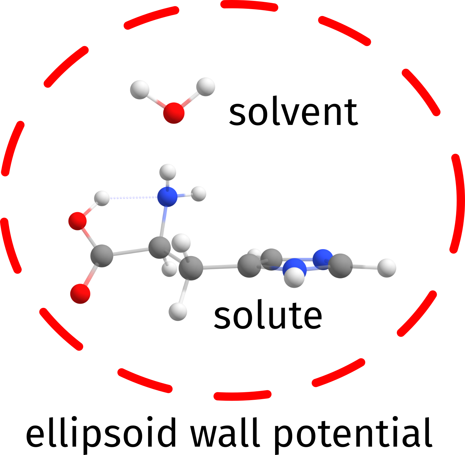
../../_images/solvator_HIS_wall.png — Fig. 7.61 A simple scheme to show how the wall potential is built to keep the solvent molecules close to the solute space.¶

A single parameter controlled by SOLVWALLFAC under the %SOLVATOR block defines how further this wall is built outside the solute. Its default value is 1.0, and increasing it to larger values will increase the default initial wall by about half the sum of the maximum dimensions of solute plus solvent for each unit.

The initial wall potential is by default not changed, unless a) the algorithm can not place a solvent, or b) the energy of the placed solvent is higher than before. Only then the walls will be updated to help allocating the next solvent molecule, and a message will be printed with the current scaling factor.

7.47.2.2. The DOCKER¶

All options related to the docking process can be controlled as usual via the %DOCKER block. Please check the section The ORCA DOCKER: An Automated Docking Algorithm for more info.

Also, all options given under the %GEOM block such as constraints and etc., will be respected during the docking of the solvent, as with the general docking, but these can only be given for the solute.

7.47.3. Controlling True Randomness¶

Both these algorithms are intrinsically dependent on random numbers, but ORCA sets a fixed random seed such that the same results are always obtained on the same machine if calculations are repeated.

In order to make both fully random, please set %SOLVATOR RANDOMSOLVATION TRUE END.

7.47.4. Vacuum Search¶

One option that might come in handy under certain conditions is to use the SOLVATOR to add the explicit solvent based on the implicit solvation information, but actually not use any implicit solvation while trying to place them.

That is useful for instance when trying to generate aggregates of solute plus solvents that can form in gas-phase only, where there will be no other solvent molecules around. That can be set with %SOLVATOR VACUUMSEARCH TRUE END and the implicit solvation method will be ignored to compute energies and gradients. In the STOCHASTIC method, the \(\epsilon_{solv}\) will be set to 1.0.

Important

By the time of the ORCA6 release, this algorithm was still not published. Publications are under preparation.

7.47.5. Complete Keyword List¶

%SOLVATOR

   #
   # general options
   #
   
   NSOLV       10   # number of explicit solvent molecules to be added.
   
   SOLVENTFILE "solvent_file_name.xyz" # a file for custom solvents.
                                       # NOT needed for the regular
                                       # solvents available via
                                       # ALPB(solvent). charge and 
                                       # multipl. can be give on the comment.
                                       
   CLUSTERMODE STOCHASTIC   # method for adding new solvent molecules.
               DOCKING      # default
               
   PRINTLEVEL  LOW
               NORMAL       # default
               HIGH
               
   RANDOMSOLV  TRUE         # make it completely random? default FALSE.
   
   FIXSOLUTE   FALSE        # keep the solute constrained? default TRUE.
   
   #
   # stochastic method
   #
                                
   USEEEQCHARGES FALSE      # use EEQ charges during the STOCHASTIC mode?
                            # default is TRUE
                            
   DROPLET       FALSE      # create a spherical droplet? default FALSE
   
   RADIUS        10         # a radius in Angstroem for the droplet.
                            # solvent molecules will be added until the
                            # target radius is reached.
   
   #
   # docking method
   #
   
   WALLFAC     1.0          # factor use to define the initial 
                            # size of the wall potential.
                            
   # all other docking options are controlled
   # as usual via the %DOCKER block.
   # flags such as !NORMALDOCK and
   # !COMPLETEDOCK will apply here as well