7.49. Fast Multipole Method
The Fast Multipole Method (FMM) algorithm was proposed in the 1980s[317], to reduce the computation time for two-centre interactions in large systems, by moving from a quadratic relationship (O(\(N^2\))) to a quasi-linear relationship (O\((Nlog(N))\)) of the computation time with the number \(N\) of particles (atoms, point charges, etc.). This algorithm is particularly useful for long-range interactions that are difficult to ignore, such as the Coulombic interaction (1/r) which is fundamental to any system but grows quadratically with the number of centers.
The FMM is used in ORCA for accelerating QMMM calculations in the scope of electrostatic embedding: FMM-QMMM (cf. Embedding Types).
7.49.1. The Octree hierarchy
There exists a lot of detailed and pedagogical literature on the subject (we recommend for instance [49] and [377]). In the following we will only describe the main parameters.
The idea of the algorithm is to divide space to handle differently short- and long-range interactions. The latter will be approximated (cf. Approximation of the Far Field interactions). To do so, the whole system is placed in a cubic box which is iteratively divided in 8 children boxes (forming levels L: \(\text{L}=0 \rightarrow \text{L}=\text{L}_{\text{max}}\)) so as to form a structure called an Octree (see Fig. Fig. 7.62).
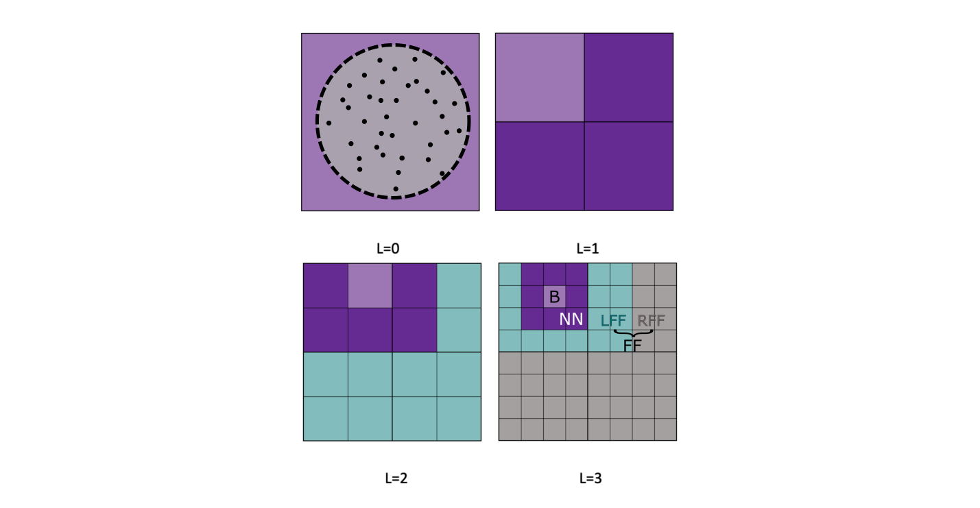
Fig. 7.62 Division of the system into boxes, schematic representation in 2D.
At the deepest level, \(\text{L}=\text{L}_{\text{max}}\), for every box, we can define a layer of nearest neighbours boxes (NN) which will be responsible for the Near-Field (NF, i.e.short-range). The electrostatic potential due to the rest of the boxes is define as the Far-Field (FF, i.e. long-range).
As visible on Figure Fig. 7.62, one can divide the FF area between a Local Far Field (LFF, green) area and a Remote Far Field area (RFF, grey), so that a recursive scheme between levels appears:
The LFF boxes are the boxes in the NF of the parent but not in the NF of the children, that represents a maximum of 189 boxes. The RFF potential is due to boxes which actually represent the FF area of the parent box of B. This means that one needs to calculate only the LFF term at every level, the rest of the potential will be inherited from the parent box.
The number of levels, \(\text{L}_{\text{max}}\), can be setup in the input directly (FMMQMMM_Levels), or will be deduced from the provided box dimension (FMMQMMM_BoxDimInp, dimension of the box at \(\text{L}_{\text{max}}\)). The second option (default) is recommended, with a box dimension around 9.0 Bohr (FMMQMMMM_BoxDimInp 9.0 ). If FMMQMMM_DoBoxDimOpt option is turned to TRUE (default), the box dimension will be reduced as much as possible while keeping the same value of \(\text{L}_{\text{max}}\), this to ensure the algorithm works optimally regarding both accuracy and efficiency.
%method
  DOFMMQMMM             True  #turn ON the use of the FMM
  FMMQMMM_BoxDimInp      9.0  #Higher boundary to set up the dimension (in Bohr!)
  FMMQMMM_DoBoxDimOpt   True  #Optimize the box dimension
end
The higher \(\text{L}_{\text{max}}\), the bigger the number of boxes: at \(\text{L}=2\) one has 64 boxes only but for \(\text{L}=6\) the code generates more than 200,000 boxes (\(8^6\)). For \(\text{L}_{\text{max}} \geq 7\), more than 2 millions boxes are generated, this can start leading to memory issues, so that the user should ensure enough memory is available (cf. Global memory use ).
7.49.2. Approximation of the Far Field interactions
In a space of origin O(0,0,0), let P (\(\textbf{r}_P\)) be the center of a charge distribution (e.g. a Gaussian overlap or a distribution of point charges). Let’s consider a point A in the vicinity of P, such that A = (q\(_A\); \(\textbf{r}_A\)), with q\(_A\) the charge of a point charge or q\(_A = -1\) if we consider a Gaussian overlap. In that case, the charge would indeed be the one of the electron situated at a position \(\textbf{r}_{AP} = \textbf{r}_{A} - \textbf{r}_{P} \) from the center of the Gaussian overlap. Similarly, let Q (\(\textbf{r}_Q\)) be the center of a charge distribution and B, a point in the vicinity of Q, such that B = (q\(_B\); \(\textbf{r}_B\)). We note \(\textbf{r}_{QP} = \textbf{r}_Q-\textbf{r}_P\).
The Coulomb interaction between A and B can be expressed as:
The name of the algorithm comes from the way the FF interactions are evaluated. It is done through a mutlipole expansion of the \(\frac{1}{|\textbf{r}_a-\textbf{r}_b|}\) term, leading to the following expression:
This series converges for well separated centers only, that is why a NF layer is required. \(R_{l,m}\) and \(I_{l,m}\) are regular and irregular solid scaled harmonics [707]:
\(Y_{l,m}\) are spherical harmonics of degree \(l\) and order \(m\). For details on the derivation of this equation see [49].
We can now introduce the multipole expansion centered in P (\(\textbf{r}_P\)), of a charge distribution \(\textbf{Q}(\textbf{r},P)\), as:
In practise:
\(\textbf{Q}\) is a vector, with elements \(Q_{l,m}\) defined by the pair of values (\(l\),\(m\)). In the case of a point charge A (q\(_A\),\(\textbf{r}\)) we have:
while for a Gaussian overlap distribution \(\braket{\mu|\nu}\) it becomes:
So that we can approximate the electrostatic interaction between a Gaussian overlap \(\braket{\mu |\nu}\) with center in \(\textbf{r}_B\) and a point charge A (q\(_A\),\(\textbf{r}_A\)) in the FF, through the following expansion:
with \(P\) and \(P\)’ the respective center of the multipole expansions, and I the interaction matrix.
The truncation parameter of the expansion, MAM, is the Maximum Angular Momentum of the underlying solid scaled harmonics. In our setup, it is the same value for the expansion of the point charges in the embedding or the Gaussian overlaps in the QM part. It can be setup through the keyword FMMQMMM_MAM. We recommend FMMQMMM_MAM = 20 to ensure a good accuracy, in the order of 0.0001-0,0001 Ha. With a lower value of MAM=15, one can usually expect a mHa (0.63 kcal.mol\(^{-1}\)) precision. However it is system dependent, so that we recommend you to start with MAM=20 and see how it behaves if you decrease it to a value of 15. The available values for MAM are in the range 1-25.
%method
  DOFMMQMMM             True  #turn ON the use of the FMM
  FMMQMMM_MAM             20   #Default Maximum Angular Momentum
end
7.49.3. The “Very” Fast Multipole Method (VFMM)
Due to the recursive scheme between levels, the FF felt in the center of a box is built by only calculating interactions with the LFF boxes at every level. The evaluation of \(V^{LFF}\) becomes the bottleneck of the algorithm. To accelerate it, an option has been implemented in which different MAM truncation parameters will be used for all the (>189) boxes in the LFF area. This option FMMQMMMM_DoVFMM is turned ON by default, but should be switched OFF whenever the MAM is smaller than 15, that would impact to much the accuracy without improving much the efficiency.
%method
  DOFMMQMMM             True  #turn ON the use of the FMM
  FMMQMMM_DoVFMM        True  #Use the Very Fast Multipole Method
end
7.49.4. Recommended input
Whenever there is an electrostatic embedding, for systems containing more than 10,000 point charges (ECM) or MM atoms (QMMM), it is recommended to turn on the FMM in order to accelerate the calculation of the electrostatic potential. However, when using heavy parallelization with more than 24 processors, the impact of enabling the Fast Multipole Method (FMM) may be negligible for small embedding size.
Caution
FMM-QMMM does not replace the QMMM keyword.
The two elements one can play on are the truncation parameter of the expansion, MAM, and the box dimension at the deepest level (\(\text{L}_{\text{max}}\)). Recommended/default parameters can be called in the keyword line directly using FMM-QMMM or by setting the parameters accordingly in the %method block:
#keyword line
! FMM-QMMM

#OR through method block

%method
  DOFMMQMMM             True  #turn ON the use of the FMM
  USEFMMQMMM            True  #turn ON the use of the FMM
  ###parameters:
  FMMQMMM_DoVFMM        True  #Use the Very Fast Multipole Method
  FMMQMMM_MAM             20  #Maximum Angular Momentum
  FMMQMMM_Levels           0  #Number of levels set to 0, will be set automatically by box dim
  FMMQMMM_BoxDimInp      9.0  #Higher boundary to set up the dimension (in Bohr!)
  FMMQMMM_DoBoxDimOpt   True  #Optimize the box dimension
end
The parameters used by the algorithm are printed in the output by default, we recomend you to check them in your first calculations:
----------------------
SHARK INTEGRAL PACKAGE
----------------------

[...]

Use FMM for one center integrals with PCs

- - - - - - - FMM PARAMETERS- - - - - - -
num PCs              75894
VFMM                  USED
MAM                   20
Input box dim        9.000
Refined box dim      5.197
Tree depth/levels      6
- - - - - - - - - - - - - - - - - - - - -
This can be turned off by modifying the relative printing options.
%method
 FMMQMMM_Printing 1 # remove FMM PARMETERS printing, default value is  2
end
7.49.5. Some examples
Call the recommanded FMM parameters through the keyword line:
!QMMM wB97X-D3BJ RIJCOSX FMM-QMMM

%qmmm
 ORCAFFFilename "file.prms"
 Embedding Electrostatic
 ChargeAlteration CS
 QMAtoms {2016:2026} end
end


*pdbfile 0 1 file.pdb
Change the MAM from 20 (value when one uses the keyword line) to 15, and use 5 levels:
!QMMM wB97X-D3BJ RIJCOSX

%method
  DOFMMQMMM             True  #turn ON the use of the FMM
  USEFMMQMMM            True  #turn ON the use of the FMM
  ###parameters:
  FMMQMMM_DoVFMM        True  #Use the Very Fast Multipole Method
  FMMQMMM_MAM             15  #Maximum Angular Momentum
  FMMQMMM_Levels           5  #number of levels
end

%qmmm
 ORCAFFFilename "file.prms"
 Embedding Electrostatic
 ChargeAlteration CS
 QMAtoms {2016:2026} end
end


*pdbfile 0 1 file.pdb
Specify the box dimension without optimizing it:
!QMMM wB97X-D3BJ RIJCOSX

%method
  DOFMMQMMM             True  #turn ON the use of the FMM
  USEFMMQMMM            True  #turn ON the use of the FMM
  ###parameters:
  FMMQMMM_DoVFMM        True  #Use the Very Fast Multipole Method
  FMMQMMM_MAM             15  #Maximum Angular Momentum
  FMMQMMM_Levels           0  #number of levels
  FMMQMMM_BoxDimInp      9.0  #Higher boundary to set up the dimension (in Bohr!)
  FMMQMMM_DoBoxDimOpt   False #Does not optimize the box dimension
end

%qmmm
 ORCAFFFilename "file.prms"
 Embedding Electrostatic
 ChargeAlteration CS
 QMAtoms {2016:2026} end
end


*pdbfile 0 1 file.pdb
Specifying the box dimension and ask to optimize it:
!QMMM wB97X-D3BJ RIJCOSX

%method
  DOFMMQMMM             True  #turn ON the use of the FMM
  USEFMMQMMM            True  #turn ON the use of the FMM
  ###parameters:
  FMMQMMM_DoVFMM        True  #Use the Very Fast Multipole Method
  FMMQMMM_MAM             15  #Maximum Angular Momentum
  FMMQMMM_Levels           0  #number of levels
  FMMQMMM_BoxDimInp      9.0  #Higher boundary to set up the dimension (in Bohr!)
  FMMQMMM_DoBoxDimOpt   True  #Optimize the box dimension
end

%qmmm
 ORCAFFFilename "file.prms"
 Embedding Electrostatic
 ChargeAlteration CS
 QMAtoms {2016:2026} end
end


*pdbfile 0 1 file.pdb