6.10. ORCA SOLVATOR: Automatic Placement of Explicit Solvent Molecules
From ORCA6, we also have a tool that can automatically place explicit solvent molecules to a given system. It can be done using two different approaches: a STOCHASTIC method which is very fast but less accurate, or a DOCKING approach which makes use of the DOCKER. The later is slower, but more accurate and is the default.
6.10.1. First Example: Adding Water to a Histidine
As a very simple initial example, let’s take a Histidine aminoacid and add three explicit water molecules at the best positions using the DOCKER and GFN2-XTB. The input to get this is as simple as:
!XTB ALPB(WATER) PAL16
%SOLVATOR NSOLV 3 END
* XYZ 0 1
  N     0.885996   -0.961304   -0.120339
  C     1.798313    0.104987    0.275069
  C     1.249714    0.744242    1.567548
  O     1.573032    1.831447    1.951866
  C     2.049102    1.187937   -0.781297
  C     2.714441    0.645674   -1.999072
  N     2.728606    1.335092   -3.185194
  C     3.401683    0.571600   -4.081842
  N     3.805612   -0.545068   -3.552995
  C     3.389082   -0.516790   -2.258890
  O     0.397674   -0.041862    2.212628
  H     0.272440   -0.853698    1.671197
  H     1.339440   -1.612664   -0.750009
  H     0.086389   -0.572348   -0.612909
  H     2.756495   -0.353470    0.548654
  H     2.661849    1.969568   -0.321790
  H     1.092545    1.646672   -1.057454
  H     2.328734    2.246496   -3.338113
  H     3.566873    0.866218   -5.098496
  H     3.616501   -1.333139   -1.602802
*
That is as simple as a regular input with the line %SOLVATOR NSOLV 3 END added. The solvent structure will be automatically taken from the implicit solvation method (in this case ALPB(WATER)), and the three water molecules will be added. The output will look like:
                       *****************
                       * ORCA Solvator *
                       *****************

Solvent chosen:                                WATER
Solvent radius:                                .... 1.69 Angs
Solvent max dimensions (x,y,z):                .... 2.73, 2.32, 1.52 Angs
Number of solvent molecules to be added:       .... 3 molecules
Method used to add the solvent:                .... docking
Number of atoms of solvent molecule:           .... 3 atoms
Coordinates of solvent in Angstroem:

   O    0.000014   0.401429   0.000000
   H    0.765192  -0.200729   0.000000
   H   -0.765206  -0.200700   0.000000

Solute radius:                                 .... 5.27 Angs
Ellipsoid potential radii:                     .... 8.37, 6.28, 5.76 Angs
where the solvent chosen is printed, together with some details about its dimensions, the number of molecules to be added and the method. The structure from the internal database is also always printed.
The process is then monitored per solvent molecule:
Adding solvent molecules to the solute         ....


      Iter       Energy      Einter          dE          Time
                  (Eh)     (kcal/mol)    (kcal/mol)     (min)
      -------------------------------------------------------
         1    -39.452446    -4.331670     -4.331670      0.26
         2    -44.544347    -4.316639      0.015031      0.34
         3    -49.636018    -4.171990      0.144649      0.40

Final radius after microsolvation:             .... 4.88 Angs
Time needed for microsolvation   :             .... 60.54 s
Final structured saved to        :             HIS.solvator.xyz

                ****ORCA-SOLVATOR TERMINATED NORMALLY****
and the final result is printed to the file Basename.solvator.xyz. There will be also an intermediate file named Basename.solvator.solventbuild.xyz with the solvent molecules added one by one.
Note
In contrast to the DOCKER, the solute is always frozen by default. Set FIXSOLUTE FALSE under the %SOLVATOR block to change that.
On the output Einter is the interaction energy obtained from the DOCKER and dE is the different between the current and the previous Einter.
In this case, the result looks like:
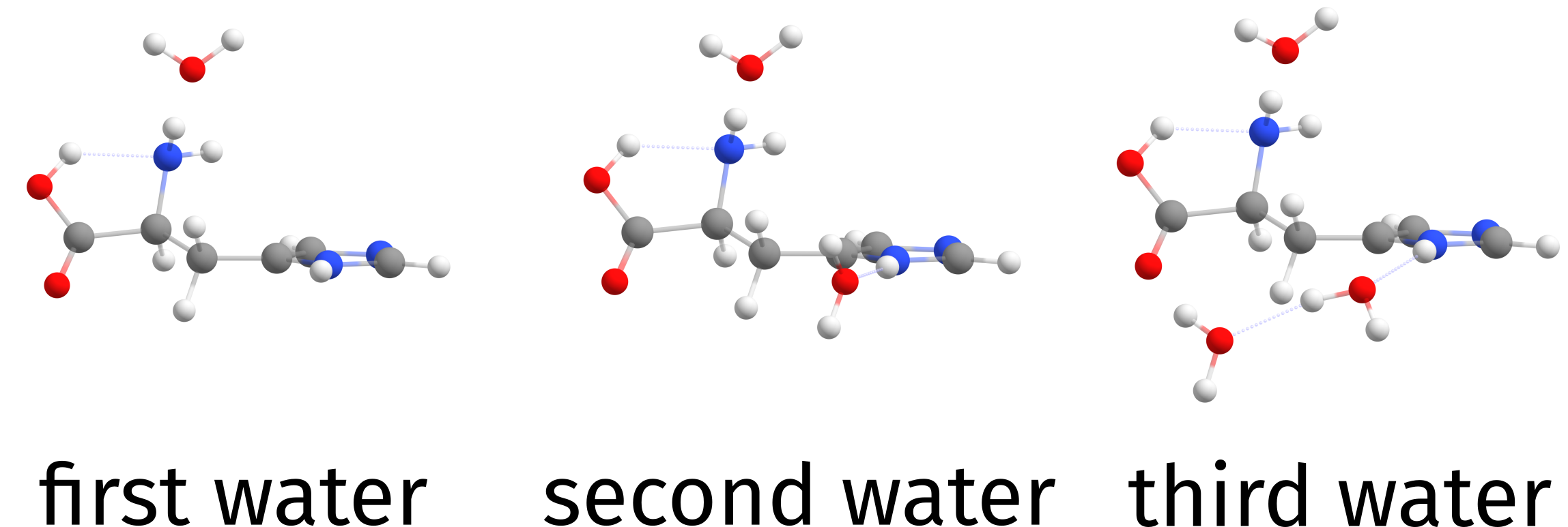
Fig. 6.34 Three water molecules added by the solvator.
Note
Currently the SOLVATOR is only working with the GFN-XTB and GFN-FF methods and the ALPB solvation model. It will be expanded later to others.
6.10.2. Other Solvents
The method itself is agnostic to the solvent, and any other could have been used. The example above with DMSO would be:
!XTB ALPB(DMSO) PAL16
%SOLVATOR NSOLV 3 END
* XYZFILE 0 1 HIS.xyz
and results in:

Fig. 6.35 Three DMSO molecules added by the solvator.
and even a custom solvent can be given in the form of a .xyz file with:
%SOLVATOR SOLVENTFILE "solvent_file_name.xyz" END
As with the docker, the charge and multiplicty can be given to the solvent if given as two integers on the comment line (default is neutral closed-shell). Since the ALPB method has a fixed number of solvents, right now one can still not give a custom epsilon value for the custom solvents, but it needs to be approximated to the next closest solvent.
As an example, let’s create a file named isopropanol.xyz with a solvent which is not on the ALPB list:
12
0 1
C         -3.79410        2.24670       -0.09622
C         -3.45574        0.76660       -0.18820
H         -2.94382        2.85306       -0.42645
H         -4.00575        2.53923        0.93817
H         -4.66172        2.49512       -0.71492
C         -4.60559       -0.10847        0.28691
H         -4.84802        0.09429        1.33594
H         -4.32886       -1.16657        0.22730
H         -5.50341        0.05251       -0.31744
O         -2.30376        0.49878        0.60542
H         -3.20686        0.51239       -1.22373
H         -2.51694        0.72259        1.52758
and run:
!XTB ALPB(ETHANOL) PAL16
%SOLVATOR SOLVENTFILE "isopropanol.xyz" NSOLV 3 END
* XYZFILE 0 1 HIS.xyz
approximating the dielectric constant of isopropanol to that of ethanol. That might look not too accurate, but the ALPB implicit solvation is also not a very good implicit solvation model anyway, so results will be quite similar.

Fig. 6.36 Three iso-propanol molecules added by the solvator.
6.10.3. The Stochastic Method for Multiple Solvents
In case you want to add a really large number of explicit solvent molecules, the STOCHASTIC mode will be significantly faster. Let’s add 100 water molecules on our target Histidine, now using CLUSTERMODE STOCHASTIC:
!XTB ALPB(WATER) PAL16
%SOLVATOR
    NSOLV       100
    CLUSTERMODE STOCHASTIC
END
* XYZFILE 0 1 HIS.xyz
The output will be somewhat different:
Solvent chosen:                                WATER
Solvent radius:                                .... 1.69 Angs
Solvent max dimensions (x,y,z):                .... 2.73, 2.32, 1.52 Angs
Number of solvent molecules to be added:       .... 100 molecules
Method used to add the solvent:                .... stochastic
Number of atoms of solvent molecule:           .... 3 atoms
Coordinates of solvent in Angstroem:

   O    0.000014   0.401429   0.000000
   H    0.765192  -0.200729   0.000000
   H   -0.765206  -0.200700   0.000000

Solute radius:                                 .... 5.27 Angs
Adding solvent molecules to the solute         ....

      Iter     Target function   Time
                  (Coulomb)     (min)
      -------------------------------
         1     -4.659435e-07     0.00
         2     -4.604606e-07     0.00
         3     -2.519684e-07     0.00
      (...)

Final radius after microsolvation:             .... 9.79 Angs
Time needed for microsolvation   :             .... 5.11 s
Final structured saved to        :             HIS_STOCHASTIC.solvator.xyz

                ****ORCA-SOLVATOR TERMINATED NORMALLY****
and in a few seconds all solvent molecules are added as can be seen from the result:

Fig. 6.37 A hundred water molecules added by the solvator.
Important
As the name says, the CLUSTERMODE STOCHASTIC is a probabilistic approach and is not nearly as accurate as the DOCKING mode! Nonetheless it is useful for quite a few applications.
6.10.4. Creating a Droplet
The regular stochastic method will create a solvation sphere around the solute following it shape and topology. In case you want to create a solvent distribution with spherical symmetry, you have to use set the DROPLET TRUE keyword, such as:
!XTB ALPB(WATER) PAL16
%SOLVATOR
    NSOLV       100
    CLUSTERMODE STOCHASTIC
    DROPLET     TRUE
END
* XYZFILE 0 1 HIS.xyz
And the result will look like:

Fig. 6.38 A hundred water molecules added by the solvator by enforcing spherical symmetry.
6.10.5. Creating a Droplet with a Defined Radius
Instead of defining the number of solvent molecules, one can also defined a maximum radius and the SOLVATOR will add as many molecules as necessary until the radius is reached. This is only compatible with CLUSTERMODE STOCHASTIC!
!XTB ALPB(WATER) PAL16
%SOLVATOR
    RADIUS      15 # in angstroem
    CLUSTERMODE STOCHASTIC
END
* XYZFILE 0 1 HIS.xyz
The output in the end shows:
Desired sovent radius:                         .... 15.00 Angs
Actual sovent radius:                          .... 15.18 Angs
Final number of solvent molecules:             .... 668 molecules
Note
The radius is taken from the centroid of the solute!
and a radius close to 15 Angstroem was achieved when 668 molecules are added:

Fig. 6.39 A droplet create with 668 water molecules to achieve a radius of approximately 15 Angstroem.
Important
All examples described above work for any other solvents, including custom ones.
Note
The default DOCKER settings for the solvator are equivalent to !QUICKDOCK. For more accurate methods use !NORMALDOCK or even !COMPLETEDOCK, however they will be much slower.
A complete list of keywords and more discussions on the topic can be found at the later section More on the ORCA SOLVATOR