6.12. Calculation of Properties

6.12.1. Population Analysis and Related Things

Atomic population related things are not real molecular properties since they are not observables. They are nevertheless highly useful for interpreting experimental and computational findings. By default, ORCA provides very detailed information about calculated molecular orbitals and bonds through Mulliken, Löwdin, and Mayer population analyses. However, as it is easy to become overwhelmed by the extensive population analysis section of the output, ORCA allows users to turn off most features.

! HF def2-SVP Mulliken Loewdin Mayer ReducedPOP

*xyz 0 1
 C  0  0  0
 O  0  0  1.13
*

The “ReducedPOP” keyword reduces the information printed out in the population analysis section, providing orbital population of each atom with percent contribution per basis function type. This is highly useful in figuring out the character of the MOs. Furthermore, one can request a printout of the MO coefficients through the output block of the input file (see section Population Analyses and Control of Output) or using the keyword “PrintMOs”

The distribution of the frontier molecular orbitals (FMOs) over the system can be requested with the “FMOPop” keyword:

! HF def2-SVP FMOPop

*xyz 0 1
 C  0  0  0
 O  0  0  1.13
*

This provides Mulliken and Loewdin population analyses on HOMO and LUMO:

----------------------------------------------
FRONTIER MOLECULAR ORBITAL POPULATION ANALYSIS
----------------------------------------------

ANALYZING ORBITALS: HOMO=   6 LUMO=   7

-------------------------------------------------------------------------
   Atom        Q(Mulliken)     Q(Loewdin)     Q(Mulliken)     Q(Loewdin) 
              <<<<<<<<<<<<HOMO>>>>>>>>>>>>   <<<<<<<<<<<<LUMO>>>>>>>>>>>>
-------------------------------------------------------------------------
   0-C         0.937186        0.906827       0.804044        0.755610
   1-O         0.062814        0.093173       0.195956        0.244390
-------------------------------------------------------------------------

Visualization of three-dimensional representation of MOs, natural orbitals, electron densities, and spin densities is usually more intuitive than examining MO coefficients and it is is described in detail in section Orbital and Density Plots. The files necessary for such visualizations can be readily generated with ORCA in various ways and then opened in visualization software such as gOpenMol and Molekel.[1] . In the following example, we briefly describe visualization of MOs.

To visualize MOs withgOpenMol, the plt file of MOs can be generated in the gOpenMol_bin format from the gbw file using orca_plot utility program or directly from the ORCA run through the %plots block of the input file:

! HF def2-SVP XYZFile

%plots Format gOpenMol_bin
       MO("CO-4.plt",4,0);
       MO("CO-8.plt",8,0);
       end
	   
*xyz 0 1
 C  0  0  0
 O  0  0  1.13
*

In this input file, the MO("CO-4.plt",4,0); command is used to evaluare MO labeled as 4 for operator 0 and then to strore it in the “CO-4.plt” file. For RHF and ROHF, one should always use operator 0. For UHF, operators 0 and 1 correspond to spin-up and spin-down orbitals, respectively.

When the produced plt files are opened with gOpenMol (see section Surface Plots for details), the textbook-like \(\pi\) and \(\pi^{\ast}\) MOs of the CO molecule are visualized as in Figure Fig. 6.40.

(a)

(b)

Fig. 6.40 (a) \(\pi\) and (b) \(\pi^\ast\) MOs of the CO molecule obtained from the interface of ORCA to gOpenMol.

If the gOpenMol_ascii file format was requested, gOpenMol conversion utility or some other tools might then be needed to convert this human-readable file to the machine-readable gOpenMol_bin format.

In order to use the interface to Molekel, an ASCII file in the Cube or Gaussian_Cube format needs to be generated. Such ASCII files can be actually transferred between platforms. The Cube format can be requested in the %plots block as:

! HF def2-SVP XYZFile
 
%plots Format Cube
       MO("CO-4.cube",4,0);
       MO("CO-8.cube",8,0);
       end

*xyz 0 1
 C  0  0  0
 O  0  0  1.13
*

To visualize MOs strored in the *.cube file, start Molekel and, via a right mouse click, load the *.xyz file and/or the *.cube file. lternatively, navigate to the surface menu, select the “gaussian-cube” format, and load the surface. For orbitals, click the “both signs” button and select a countour value in the “cutoff” field. Then, click “create surface”. The colour schemes and other fine details of the plots can be easily adjusted as desired. Finally, create files via the “snapshot” feature of Molekel. Figure Fig. 6.41 demonstrates a Molekel variant of Figure Fig. 6.40.

(a)

(b)

Fig. 6.41 (a) \(\pi\) and (b) \(\pi^\ast\) MOs of the CO molecule obtained from the interface of ORCA to Molekel.

It is worth noting that there are several other freeware programs, such as UCSF CHIMERA, that can read Gaussian_Cube files and provide high-quality plots.

In some situations, visualization of the electronic structure in terms of localized molecular orbitals might be quite helpful. As unitary transformations among occupied orbitals do not change the total wavefunction, such transformations can be applied to the canonical SCF orbitals with no change of the physical content of the SCF wavefunction. The localized orbitals correspond more closely to the pictures of orbitals that chemists often enjoy to think about. Localized orbitals according to the Pipek-Mezey population-localization scheme are quite easy to compute. For example, the following run reproduces the calculations reported by Pipek and Mezey in their original paper for the N\(_{2}\)O\(_{4}\) molecule.

! HF STO-3G Bohrs

%loc 
     LocMet  PipekMezey # localization method. Choices:
                            # PipekMezey (=PM)
                            # FosterBoys (=FB)
     T_Core  -1000      # cutoff for core orbitals
     Tol     1e-8       # conv. Tolerance (default=1e-6)
     MaxIter 20         # max. no of iterations (def. 128)
     end

*xyz 0 1
 N    0.000000   -1.653532   0.000000
 N    0.000000    1.653532   0.000000
 O   -2.050381   -2.530377   0.000000
 O    2.050381   -2.530377   0.000000
 O   -2.050381    2.530377   0.000000
 O    2.050381    2.530377   0.000000
*

Based on the output file of this job, localized MOs consist of six core like orbitals (one for each N and one for each O), two distinct lone pairs on each oxygen, a \(\sigma\)- and a \(\pi\)-bonding orbital for each N-O bond and one N-N \(\sigma\)-bonding orbital which corresponds to the dominant resonance structure of this molecule. You will also find a file with the extension .loc in the directory where you run the calculation. Like the standard gbw file, it can used to extract files for plotting or as input for another calculation (warning! The localized orbitals have no well defined orbital energy. If you do use them as input for another calculation use GuessMode=CMatrix in the %scf block).

If you have access to a version of the gennbo program from Weinhold’s group[2], you can also request natural population analysis and natural bond orbital analysis. The interface is elementary and is invoked through the keywords NPA and NBO, respectively:

! HF def2-SVP NPA XYZFile 

* xyz 0 1
  C  0  0  0
  O  0  0  1.13
*

If you choose simple NPA, then you will only obtain a natural population analysis. When NBO is chosen instead, the natural bond orbital analysis will also be carried out. ORCA leaves a FILE.47 file on disk. This file can be edited to use all of the features of the gennbo program in the stand-alone mode. Please refer to the NBO manual for further details.

6.12.2. Absorption and Fluorescence Bandshapes using ORCA_ASA

Please also consider using the more recent ORCA_ESD, described in Section Excited State Dynamics, to compute bandshapes.

Bandshape calculations are nontrivial but can be achieved with ORCA using the procedures described in section Simulation and Fit of Vibronic Structure in Electronic Spectra, Resonance Raman Excitation Profiles and Spectra with the orca_asa Program. Starting from version 2.80, analytical TD-DFT gradients are available, which make these calculations quite fast and applicable without expert knowledge to larger molecules.

Note

• Functionals with somewhat more HF exchange produce better results and are not as prone to “ghost states” as GGA functionals unfortunately are!

• Calculations can be greatly sped up by the RI or RIJCOSX approximations!

• Analytic gradients for the (D) correction and hence for double-hybrid functionals are NOT available.

In a nutshell, let us look into the H\(_{2}\)CO molecule. First we generate some Hessian (e.g. BP86/SV(P)). Then we run the job that makes the input for the orca_asa program. For example, let us calculate the five lowest excited states:

! aug-cc-pVDZ BHandHLYP TightSCF NMGrad 

%tddft nroots 5 end

# this is ASA-specific input
%rr    states 1,2,3,4,5
       HessName "Test-ASA-H2CO-freq.hess"
       ASAInput True
       end 

*int 0 1
 C 0 0 0  0   0     0 
 O 1 0 0  1.2 0     0
 H 1 2 0  1.1 120   0
 H 1 2 3  1.1 120 180
*

The ORCA run will produce a file Test-ASA-H2CO.asa.inp that is an input file for the program that generates various spectra. It is an ASCII file that is very similar in appearance to an ORCA input file:

#
# ASA input
#
%sim     model IMDHO
         method Heller

         AbsRange     25000.0,  100000.0
         NAbsPoints   1024

         FlRange      25000.0,  100000.0
         NFlPoints    1024

         RRPRange     5000.0,  100000.0
         NRRPPoints   1024

         RRSRange        0.0,    4000.0
         NRRSPoints   4000

         # Excitation energies (cm**-1) for which rR spectra will
         # be calculated. Here we choose all allowed transitions
         # and the position of the 0-0 band
         RRSE 58960, 66884, 66602

         # full width half maximum of Raman bands in rR spectra
         # (cm**-1):
         RRS_FWHM 10.0

         AbsScaleMode Ext
         FlScaleMode  Rel
         # RamanOrder=1 means only fundamentals. For 2 combination
         # bands and first overtones are also considered, for 3
         # one has second overtones etc.
         RamanOrder   1

         # E0 means the adiabatic excitation energy
         # EV would mean the vertical one. sprints vertical
         # excitations in the TD-DFT output but for the input into
         # the ASA program the adiabatic excitation energies are
         # estimated. A rigorous calculation would of course in-
         # volve excited state geometry optimization
         EnInput E0

         CAR   0.800
         end

# These are the calculated electronic states and transition moments
# Note that this is in the Franck-Condon approximation and thus
# the transition moments have been calculated vertically
$el_states
5
   1 32200.79   100.00    0.00    -0.0000   0.0000  -0.0000
   2 58960.05   100.00    0.00     0.0000  -0.4219   0.0000
   3 66884.30   100.00    0.00    -0.0000   0.4405   0.0000
   4 66602.64   100.00    0.00    -0.5217  -0.0000   0.0000
   5 72245.42   100.00    0.00     0.0000   0.0000   0.0000

# These are the calculated vibrational frequencies for the totally
# symmetric modes. These are the only ones that contribute. They
# correspond to x, H-C-H bending, C=O stretching and C-H stretching
# respectively
$vib_freq_gs
3
    1     1462.948534
    2     1759.538581
    3     2812.815170

# These are the calculated dimensional displacements for all
# electronic states along all of the totally symmetric modes.
$sdnc
3 5
                   1          2          3          4          5
      1      -0.326244   0.241082  -0.132239   0.559635   0.292190
      2      -1.356209   0.529823   0.438703   0.416161   0.602301
      3      -0.183845   0.418242   0.267520   0.278880   0.231340

After setting NAbsPoints variable and spectral ranges in this file to the desired values, we invoke orca_asa as:

orca_asa Test-ASA-H2CO.asa.inp

This produces the following output:

******************
                                    * O R C A  A S A *
                                    ******************

                    --- A program for analysis of electronic spectra ---


Reading file: Test-ASA-H2CO.asa.inp ... done


         **************************************************************
         *        GENERAL CHARACTERISTICS OF ELECTRONIC SPECTRA        *
         **************************************************************

--------------------------------------------------------------------------------
  State      E0           EV       fosc    Stokes shift  Effective Stokes shift
          (cm**-1)     (cm**-1)              (cm**-1)           (cm**-1)
--------------------------------------------------------------------------------
    1:     30457.24   32200.79   0.000000      0.00                0.00
    2:     58424.56   58960.05   0.031879      0.00                0.00
    3:     66601.54   66884.30   0.039422      0.00                0.00
    4:     66111.80   66602.64   0.055063      0.00                0.00
    5:     71788.55   72245.42   0.000000      0.00                0.00


--------------------------------------------------------------------------------------------------
                                BROADENING PARAMETETRS (cm**-1)
--------------------------------------------------------------------------------------------------
                 Intrinsic                                    Effective
   State   --------------------------  --------------------------------------------------------
                                                    Sigma                         FWHM
            Gamma    Sigma    FWHM      ---------------------------   ---------------------------
                                           0K       77K     298.15K      0K       77K     298.15K
--------------------------------------------------------------------------------------------------
    1:     100.00     0.00   200.00        0.00      0.00      0.00    200.00    200.00    200.00
    2:     100.00     0.00   200.00        0.00      0.00      0.00    200.00    200.00    200.00
    3:     100.00     0.00   200.00        0.00      0.00      0.00    200.00    200.00    200.00
    4:     100.00     0.00   200.00        0.00      0.00      0.00    200.00    200.00    200.00
    5:     100.00     0.00   200.00        0.00      0.00      0.00    200.00    200.00    200.00


Calculating absorption spectrum   ...
The maximum number of grid points ... 5840
Time for absorption               ...       9.569 sec (=   0.159 min)
Writing file: Test-ASA-H2CO.asa.abs.dat ... done
Writing file: Test-ASA-H2CO.asa.abs.as.dat ... done

Generating vibrational states up to the  1-th(st) order  ...   done
Total number of vibrational states                       ...      3

Calculating rR profiles for all vibrational states up to the 1-th order
State 1 ...
The maximum number of grid points ... 6820
Resonance Raman profile is done
State 2 ...
The maximum number of grid points ... 6820
Resonance Raman profile is done
State 3 ...
The maximum number of grid points ... 6820
Resonance Raman profile is done
Writing file: Test-ASA-H2CO.asa.o1.dat... done
Writing file: Test-ASA-H2CO.asa.o1.info... done

Calculating rR spectra involving vibrational states up to the 1-th(st) order
State    1 ... done
State    2 ... done
State    3 ... done

Writing file: Test-ASA-H2CO.asa.o1.rrs.58960.dat      ... done
Writing file: Test-ASA-H2CO.asa.o1.rrs.58960.stk      ... done
Writing file: Test-ASA-H2CO.asa.o1.rrs.66884.dat      ... done
Writing file: Test-ASA-H2CO.asa.o1.rrs.66884.stk      ... done
Writing file: Test-ASA-H2CO.asa.o1.rrs.66602.dat      ... done
Writing file: Test-ASA-H2CO.asa.o1.rrs.66602.stk      ... done
Writing file: Test-ASA-H2CO.asa.o1.rrs.as.58960.dat   ... done
Writing file: Test-ASA-H2CO.asa.o1.rrs.as.58960.stk   ... done
Writing file: Test-ASA-H2CO.asa.o1.rrs.as.66884.dat   ... done
Writing file: Test-ASA-H2CO.asa.o1.rrs.as.66884.stk   ... done
Writing file: Test-ASA-H2CO.asa.o1.rrs.as.66602.dat   ... done
Writing file: Test-ASA-H2CO.asa.o1.rrs.as.66602.stk   ... done
Writing file: Test-ASA-H2CO.asa.o1.rrs.all.xyz.dat    ... done

TOTAL RUN TIME: 0 days 0 hours 1 minutes 17 seconds 850 msec

The computed vibrationally resolved absorption spectrum is plotted as shown in Figure Fig. 6.42.

Fig. 6.42 The computed vibrationally resolved absorption spectrum of the H\(_{2}\)CO molecule

The computed fluorescence spectrum of the lowest energy peak is plotted as shown in Figure Fig. 6.43. This peak corresponds to S2. Although it is not realistic, it is sufficient for illustrative purposes.

Fig. 6.43 The computed fluorescence spectrum of the lowest energy peak of the H\(_{2}\)CO molecule

The computed Resonance Raman (rR) excitation profiles of the three totally symmetric vibrational modes are plotted as shown in Figure Fig. 6.44.

Fig. 6.44 The computed Resonance Raman excitation profiles of the three totally symmetric vibrational modes of the H\(_{2}\)CO molecule

As might be expected, the dominant enhancement occurs under the main peaks for the C\(=\)O stretching vibration. Higher energy excitations particularly enhance the C-H vibrations. The computed rR spectra at the vertical excitation energies are provided in Figure Fig. 6.45.

Fig. 6.45 The computed Resonance Raman spectra at the vertical excitation energies of the H\(_{2}\)CO molecule

In this toy example, the dominant mode is the C\(=\)O stretching, and the spectra look similar for all excitation wavelengths. However, electronically excited states are mostly of different natures, yielding drastically different rR spectra. Thus, rR spectra serve as powerful fingerprints of the electronic excitation being studied. This is also true even if the vibrational structure of the absorption band is not resolved, which is usually the case for large molecules.

The orca_asa program is much more powerful than described in this section. Please refer to section Simulation and Fit of Vibronic Structure in Electronic Spectra, Resonance Raman Excitation Profiles and Spectra with the orca_asa Program for a full description of its features. The orca_asa program can also be interfaced to other electronic structure codes that deliver excited state gradients and can be used to fit experimental data. It is thus a tool for experimentalists and theoreticians at the same time!

6.12.3. IR/Raman Spectra, Vibrational Modes and Isotope Shifts

6.12.3.1. IR Spectra

**There were significant changes in the IR printing after ORCA 4.2.1!**

IR spectral intensities are calculated automatically in frequency runs. Thus, there is nothing to control by the user. Consider the following job:

! OPT FREQ BP86 def2-SVP

*xyz 0 1
 O    0.000000    0.000000    0.611880
 C    0.000000    0.000000   -0.596849
 H    0.952616    0.000000   -1.209311
 H   -0.952616    0.000000   -1.209311
*

which gives the following output:

-----------
IR SPECTRUM
-----------

 Mode   freq       eps      Int      T**2         TX        TY        TZ
       cm**-1   L/(mol*cm) km/mol    a.u.
----------------------------------------------------------------------------
  6:   1146.68   0.000341    1.73  0.000093  (-0.000000 -0.009640  0.000000)
  7:   1224.67   0.002004   10.13  0.000511  ( 0.022596  0.000000  0.000000)
  8:   1485.77   0.001002    5.07  0.000211  ( 0.000000 -0.000000  0.014510)
  9:   1806.49   0.020286  102.51  0.003504  ( 0.000000 -0.000000  0.059197)
 10:   2769.13   0.014010   70.80  0.001579  ( 0.000000  0.000000  0.039734)
 11:   2812.52   0.039321  198.71  0.004363  ( 0.066052 -0.000000 -0.000000)

The first column (‘Mode’) labels vibrational modes that increase in frequency from top to bottom.” The next column provides vibrational frequencies. The molar absorption coefficient \(\varepsilon\) of each mode is listed in the “eps” column. This quantity is directly proportional to the intensity of a given fundamental in an IR spectrum, and thus it is used by the orca_mapspc utility program as the IR intensity.

The values under “Int” are the integrated absorption coefficient[3], and the “T**2” column lists the norm of the transition dipole derivatives, already including the vibrational part.

To obtain a plot of the spectrum, the orca_mapspc utility can be run calling the output file as:

orca_mapspc Test-Freq-H2CO.out ir -w25

or calling the Hessian file as:

orca_mapspc Test-Freq-H2CO.hess ir -w25

The basic options of orca_mapspc are listed below:

-w  : a value for the linewidth (gaussian shape, fwhm)
-x0 : start value of the spectrum in cm**-1
-x1 : end value of the spectrum in cm**-1
-n  : number of points to use

To see its options in detail, call orca_mapspc without any input. The above orca_mapspc runs of the H\(_2\)CO molecule provide Test-NumFreq-H2CO.out.ir.dat file that contains intensity and wavenumber columns. Therefore, this file can serve as input for any graph plotting program. The plot of the computed IR spectrum of the H\(_2\)CO molecule obtained with the above ORCA run is as given in Figure Fig. 6.46.

Fig. 6.46 The predicted IR spectrum of the H\(_2\)CO molecule plotted using the file generated by the orca_mapspc tool.

6.12.3.2. Overtones, Combination bands and Near IR spectra via NEARIR

Overtones and combination bands can also be incorporated to the computed IR or Near IR spectrum for completeness. The intensities of these bands are strongly dependent on anharmonic effects. ORCA can include these effects by means of the VPT2 approach [77]. The full cubic force field, anharmonic corrections to overtones and combination bands, and a broad range of methods are available in the orca_vpt2 module (see section Anharmonic Analysis and Vibrational Corrections using VPT2/GVPT2 and orca_vpt2).

In particular, the NEARIR keyword calls a simpler semidiagonal approach, including only two modes (\(i\) and \(j\), also refered as 2MR-QFF in [74, 895]) and force constants up to cubic order (\(k_{iij}\), \(k_{iji}\) and \(k_{iii}\)). For now, only the intensities are corrected for anharmonic effects - frequencies are not.

6.12.3.2.1. Overtones and Combination bands

Since the calculation of these terms scale with \(N_{modes}^2\), it can quickly become too expensive, thus we use by default the semiempirical GFN2-xTB [332] to compute the energies and dipole moments necessary to the higher order derivatives (which can be changed later). To request this, simply add !NEARIR in the main input. An example input for computing the fundamentals of toluene using B2PLYP double-hybrid functional and for computing the anharmonics using XTB is as follows:

! TightOPT NumFREQ RI-B2PLYP def2-TZVP def2-TZVP/C RIJCOSX NEARIR
 
*xyzfile 0 1 toluene.xyz

Note

These anharmonic corrections are very sensitive to the geometry. Therefore, perform a conservative geometry optimization (at least TightOPT) whenever possible.

In the output, the characteristics of the regular IR spectrum are printed first. Then, the characteristics of overtones and combination bands are provided similarly to the fundamentals, as follows:

-------------------------------
OVERTONES AND COMBINATION BANDS
-------------------------------

Mode      freq       eps       Int      T**2        TX        TY        TZ
         cm**-1   L/(mol*cm)  km/mol    a.u.
------------------------------------------------------------------------------
6+6:      64.71    0.000994    5.02   0.004792  (-0.009428 -0.066232  0.017796)
6+7:      241.83   0.000022    0.11   0.000028  (-0.005268  0.000255  0.000638)
6+8:      375.36   0.000048    0.24   0.000040  (-0.000740  0.001917  0.006007)
6+9:      442.49   0.000000    0.00   0.000000  ( 0.000010  0.000001  0.000001)
6+10:     506.37   0.000003    0.01   0.000002  ( 0.001078 -0.000061  0.000799)
(...)

The “Mode” column shows the overtones, such as 6+6, and combination bands, such as 6+7 and 6+8. These new quantities are automatically detected and incorporated in the IR spectrum when the output file is called with the orca_mapspc utility as follows:

orca_mapspc toluene-nearir.out ir -w25

From the file orca_mapspc provided, the IR spectrum can be plotted as shown in Figure Fig. 6.47.

Fig. 6.47 Calculated and experimental infrared spectrum of toluene in gas phase. While the red plot includes only the fundamentals, the blue plot includes also overtones and combination bands. The grey dashed plot is the experimental gas-phase spectrum obtained from the NIST database. The theoretical frequencies were scaled following literature values [442]

“Benzene fingers”, i.e., overtones and combination bands of the ring, are recovered in the computed spectrum. Note that the frequencies were scaled using literature values [442], and are not yet corrected using VPT2.

6.12.3.2.2. Near IR spectra

Let us simulate near IR spectrum of methanol in CCl\(_4\), as published by Bec and Huck [82], using B3LYP for fundamentals, XTB for overtones, and CPCM for solvation. The input is as follows:

! TightOPT FREQ B3LYP def2-TZVP RIJCOSX NEARIR CPCM(CCl4)

*xyz 0 1
 O      0.39517      4.38840     -0.00683
 C     -0.50818      3.29837      0.00221
 H     -0.11943      5.18771      0.19752
 H      0.03977      2.38083     -0.22470
 H     -1.27919      3.45664     -0.75583
 H     -0.96616      3.21170      0.99058
*

Calling the output with orca_mapspc by setting final point to about \(8000 cm^{-1}\) in order to extend the spectrum to the near IR region, i.e.,

orca_mapspc toluene-nearir.out ir -w25 -x18000

one can simulate the spectrum from the generated “toluene-nearir.dat” file. As seen in Figure Fig. 6.48 the computed spectrum plotted with scaled computational frequencies (not yet corrected using VPT2) according to [442] agrees reasonably well with the experimental spectrum.

Fig. 6.48 Calculated and experimental near IR spectrum of methanol in CCl\(_4\). The blue plot is for overtones; the red plot is for combination bands; and the grey dashed plot is the experimental spectrum. Theoretical frequencies were scaled according to literature values [442].

6.12.3.2.3. Using other methods for the VPT2 correction

To compute overtones with the method chosen for the calculation of the fundamentals, one needs only to set XTBVPT2 option in the %freq block to false, i.e.,

%freq XTBVPT2 False end

To set a different method for the calculation of overtones and combinations than used for the calculation of fundamentals, one needs first to perform a frequency calculation, then call the resulting Hessian file in %geom block, and activate the PRINTTHERMOCHEM flag (see section Thermochemistry for details), i.e.,

! BP86 def2-TZVP NEARIR CPCM(CCl4) PRINTTHERMOCHEM

%geom INHESSNAME "methanol.hess" end
%freq XTBVPT2 False end

*xyzfile 0 1 methanol_opt.xyz

In this example, the fundamental modes are read from the “methanol.hess” file, but the anharmonics and intensities of the overtones and combinations are computed using BP86. Any combination of methods, such as B3LYP/BP86 and B2PLYP/AM1, is allowed. Note that this description is an approximation to full VPT2 or GVPT2. For a more complete treatment, see the VPT2 module described in section Anharmonic Analysis and Vibrational Corrections using VPT2/GVPT2 and orca_vpt2.

By default, a step size of 0.5 in dimensionless normal mode unit is used during the numerical calculations. This can be changed by setting DELQ in the %freq block:

%freq
    XTBVPT2 False
    DELQ    0.1
end

The complete list of options related to VPT2 and in general frequency calculations can be found in Sec. Frequency calculations - numerical and analytical.

6.12.3.3. Vibrational Circular Dichroism (VCD) Spectra

Vibrational circular dichroism spectrum calculations are implemented analytically at the SCF (HF or DFT) level following the derivation of Weigend and coworkers. [715] The basic usage is shown in the following example:

# AnFreq + doVCD triggers the VCD calculation
! AnFreq B3LYP def2-SVP

%freq 
  doVCD true 
end

*xyz 0 1
  C      1.231429   -0.226472   -0.084960
  C     -0.061893    0.507641    0.134338
  C     -1.358912   -0.147897    0.084831
  O     -0.902881    0.641038   -0.969176
  H      1.070541   -1.118875   -0.689778
  H      1.672013   -0.522768    0.869009
  H      1.946503    0.413187   -0.605194
  H      0.017832    1.411161    0.734623
  H     -1.417896   -1.212878   -0.118068
  H     -2.196737    0.255864    0.644375
*

Note that in addition to the Hessian, the VCD calculation requires the magnetic field response using GIAOs and the electric field response with the field origin placed at (0,0,0). The latter matches the hard-coded magnetic field gauge origin in the GIAO case and is necessary to ensure gauge-invariance of the results. ORCA does all of this automatically but it means that if VCD is requested together with electric and/or magnetic properties in the same job, the field origins cannot be changed.

Other keywords that influence the VCD calculation include GIAO_1el and GIAO_2el in %eprnmr and CutOffFreq in %freq. Note also that VCD cannot be computed with NumFreq.

6.12.3.4. Raman Spectra

In order to predict Raman spectrum of a compound, derivatives of the polarizability with respect to the normal modes must be computed. Thus, if a numerical frequency run (!NumFreq) is combined with a polarizability calculation, the Raman characteristics will be automatically calculated.

Consider the following example:

! OPT NumFreq RHF STO-3G TightSCF SmallPrint

%elprop Polar 1 end

*xyz 0 1
 C    0.000000    0.000000   -0.533905
 O    0.000000    0.000000    0.682807
 H    0.000000    0.926563   -1.129511
 H    0.000000   -0.926563   -1.129511
*

The output provides the Raman scattering activity
(in \(Å^4\)/AMU)[630] and the Raman depolarization ratio of each mode:

--------------
RAMAN SPECTRUM
--------------

 Mode    freq (cm**-1)   Activity   Depolarization
-------------------------------------------------------------------
   6:      1277.66      0.010363      0.750000
   7:      1397.45      3.059009      0.750000
   8:      1767.01     16.386535      0.707349
   9:      2099.21      6.701894      0.075708
  10:      3499.49     38.643829      0.186526
  11:      3645.45     24.496534      0.750000

The ORCA run generates also a .hess file that includes polarizability derivatives and Raman activities. The effect of isotope substitution on the Raman activities can be computed using the .hess file.

As in the IR spectrum case, orca_mapspc provides a .dat file for plotting the computed Raman spectrum:

orca_mapspc Test-NumFreq-H2CO.out raman -w50

The Raman spectrum of H\(_2\)CO plotted by using the corresponding .dat file is as given in Figure Fig. 6.49.

Fig. 6.49 Calculated Raman spectrum of H\(_2\)CO at the STO-3G level plotted using the .dat generated by the orca_mapspc utility from numerical frequencies and Raman activities.

It is worth noting that Raman scattering activity \(S_i\) of each mode \(i\) is related to but not directly equal to the Raman intensity \(I_i\) of the corresponding mode, which is dependent on the excitation line \(\nu_0\) of the laser used in the Raman measurement(for Nd:YAG laser: \(\nu_0\) = 1064 nm = 9398.5 cm\(^{-1}\)). To obtain significantly better agreement between experimental and simulated Raman spectra, \(I_i\) of each mode needs to be computed with the following formula:

\[ I_i = \frac{f(\nu_0 - \nu_i)^4 S_i}{\nu_i [1 - \exp(-h c \nu_i / k T)]} \]

where \(f\) is a normalization constant common for all modes; \(h\), \(c\), \(k\), and \(T\) are Planck’s constant, speed of light, Boltzmann’s constant, and temperature, respectively.

Note

• The Raman module works only when the polarizabilities are calculated analytically. Hence, only the methods, for which the analytical derivatives w.r.t. to external fields are implemeted, can be used.

• Raman calculations take significantly longer than IR calculations due to the extra effort of calculating the polarizabilities at all displaced geometries. Since the latter step is computationally as expensive as the solution of the SCF equations you have to accept an increase in computer time by a factor of \(\approx\) 2.

6.12.3.5. Resonance Raman Spectra

Resonance Raman spectra (NRVS) and excitation profiles can be predicted or fitted using the procedures described in section Simulation and Fit of Vibronic Structure in Electronic Spectra, Resonance Raman Excitation Profiles and Spectra with the orca_asa Program. An example for obtaining the necessary orca_asa input is described in section Absorption and Fluorescence Bandshapes using ORCA_ASA.

6.12.3.6. NRVS Spectra

The details of the theory and implementation of NRVS spectrum are as described in ref. [676, 679]. The NRVS spectrum of \({iron-containing}\) \({molecules}\) can be simply calculated calling .hess file of a previous frequency calculation with the orca_vib utility. The output file of this utility can then be called with orca_mapspc utility to produce a .dat file for plotting the spectrum:

orca_vib MyJob.hess > MyJob.vib.out
orca_mapspc MyJob.vib.out NRVS

For a the ferric-azide complex [679], the computed and experimental NRVS spectra are provided in Figure Fig. 6.50.

Fig. 6.50 Experimental (a, black curve), fitted (a, red) and simulated (b) NRVS spectrum of the Fe(III)-azide complex obtained at the BP86/TZVP level (T \(=\) 20 K). Bar graphs represent the corresponding intensities of the individual vibrational transitions. The blue curve represents the fitted spectrum with a background line removed.

As for the calculation of resonance Raman spectra described in section Simulation and Fit of Vibronic Structure in Electronic Spectra, Resonance Raman Excitation Profiles and Spectra with the orca_asa Program, the DFT estimations are usually excellent starting points for least-square refinements.

Below we describe the procedure for computing such NRVS spectra on the \({\text{Fe(SH)}}_{4}^{1-}\) complex with the BP86 functional, which typically provides good NRVS spectra. One needs first to optimize the geometry of the complex and compute its vibrational structure:

! OPT FREQ BP86 def2-TZVP TightSCF SmallPrint
 
*xyz -1 6
 Fe     -0.115452      0.019090     -0.059506
 S      -0.115452      1.781846      1.465006
 S      -0.115452     -1.743665      1.462801
 S      -1.908178     -0.072782     -1.518702
 S       1.560523      0.154286     -1.656664
 H       0.410700      2.760449      0.687716
 H      -0.674147     -2.708278      0.690223
 H      -2.905212      0.345589     -0.699907
 H       2.647892     -0.211681     -0.932926
*

Now run the orca_vib utility on the .hess file generated by this job to obtain an output file that can be used with orca_mapspc utility:

orca_vib Test-FeIIISH4-NumFreq.hess > Test-FeIIISH4-NumFreq.out
orca_mapspc Test-FeIIISH4-NumFreq.out NRVS

This orca_mapspc run generates Test-FeIIISH4-NumFreq.nrvs.dat file in the xy-format. This file contains phonon energy (x, in cm\(^{-1}\)) and NRVS intensity (y, in atomic units) and thus can be directly used for visualizing the spectrum.

The corresponding NRVS spectrum is given in Figure Fig. 6.51 together with the computational IR spectrum on the same frequency scale. NRVS reports the Doppler broadening of the Moessbauer signal due to resonant scattering of phonons (vibrations) dominated by the movements of Fe nuclei. This is a valuable addition to IR spectrum where the modes have very small intensities.

Fig. 6.51 (a) Theoretical IR spectrum of \({\text{Fe(SH)}}_{4}^{1-}\) and arrow-pictures of the highest intensity modes around the peak maxima. (b) The corresponding NRVS scattering spectrum.

6.12.3.7. Animation of Vibrational Modes

For describing how to animate vibrational modes and generate their “arrow-pictures”, let us perform a frequency calculation on H\(_2\)CO:

! OPT FREQ RHF STO-3G

*xyz 0 1
 C    0.000000    0.000000   -0.533905
 O    0.000000    0.000000    0.682807
 H    0.000000    0.926563   -1.129511
 H    0.000000   -0.926563   -1.129511
*

The output of this job provides vibrational characteristics:

Mode      freq       eps       Int    T**2         TX        TY        TZ
         cm**-1   L/(mol*cm) km/mol    a.u.
----------------------------------------------------------------------------
6:       1278.37   0.001222    6.18  0.000298  (-0.017272  0.000000  0.000000)
7:       1397.26   0.005844   29.53  0.001305  ( 0.000000  0.036128  0.000000)
8:       1767.02   0.000828    4.18  0.000146  (-0.000000  0.000000 -0.012089)
9:       2099.24   0.001668    8.43  0.000248  ( 0.000000 -0.000000  0.015749)
10:      3498.54   0.000356    1.80  0.000032  ( 0.000000 -0.000000 -0.005636)
11:      3645.47   0.003922   19.82  0.000336  (-0.000000  0.018322  0.000000)

This output can be directly opened with ChemCraft to visualize normal modes of H\(_2\)CO and to extract their arrow-pictures representing the direction of nuclear movements as shown in Figure Fig. 6.52. As an example, one can infer from this figure that the 1397 cm\(^{-1}\) mode corresponds to a rocking vibration.

Fig. 6.52 Normal modes of H\(_2\)CO with arrows indicating magnitude and direction of nuclear motions and the associated vibrational frequencies in cm\(^{-1}\) obtained from ORCA output file through the use of ChemCraft

In order to animate vibrational modes and to create their “arrow-pictures” by using free program packages like gOpenMol, the small utility program orca_pltvib can be used. This utility program generates a series of files from an ORCA output file of a frequency run, which can be openned with molecular visualization programs. The usage of orca_pltvib is as follows:

orca_pltvib Test-FREQ-H2CO.out [list of vibrations or all]

For example, let us want to animate the 1397 cm\(^{-1}\) mode labeled as 7:

orca_pltvib Test-FREQ-H2CO.out 7

This call will generate the Test-FREQ-H2CO.out.v007.xyz file. Open gOpenMol and read this file (Import->coords) in Xmol format. Then, go to the Trajectory->Main menu and import again the file in Xmol format. Now you are able to animate the mode. In order to generate a printable picture, press Dismiss and then type lulVectorDemo {4 0.1 black} into the gOpenMol command line window. The generated picture (see Figure Fig. 6.53) demonstrates that this mode corresponds to a rocking vibration.

Fig. 6.53 The 1397 cm\(^{-1}\) mode of the H\(_2\)CO molecule as obtained from the interface of ORCA to gOpenMol and the orca_pltvib tool to create the animation file.

The appearence of the arrows can also be modified as described in the web tutorial of gOpenMol.

6.12.3.8. Isotope Shifts

The calculated isotope shifts greatly aid in the identification of vibrations, the interpretation of experiments, and the assessment of the reliability of the calculated vibrational normal modes. It would be a very bad practice to recalculate the Hessian for investigating isotope shift since Hessian calculations are typically expensive, and the Hessian itself is independent of the masses. Below we describe how to find the isotope effect without recomputing the Hessian.

Let us suppose that you have calculated a Hessian as in the example discussed above, and you want to predict the effect of \(^{18}\)O substitution. In this case you can use the small utility program orca_vib. First of all you need to edit the masses given in the .hess file by hand. For the example given above, the .hess file is as follows:

$orca_hessian_file
......................
$hessian
12
... the cartesian Hessian in Eh/bohr**"

$vibrational_frequencies
12

...the vibrational frequencies (in cm-1) as in the output

$normal_modes
12 12
... the vibrational normal modes in Cartesian displacements
#
# The atoms: label  mass x  y  z
# !!!!!!!!!!!!!!!!!!!!!!!!!!!!!!!!!!!!!!
#   Here we have changed 15.999 for oxygen into
#   18.0  in order to see the oxygen 18 effects
# !!!!!!!!!!!!!!!!!!!!!!!!!!!!!!!!!!!!!!!!!!!
$atoms
4
 C     12.0110      0.000000     0.000000    -1.149571
 O     18.0000     -0.000000    -0.000000     1.149695
 H      1.0080     -0.000000     1.750696    -2.275041
 H      1.0080     -0.000000    -1.750696    -2.275041

$actual_temperature
  0.000000

$dipole_derivatives
12

... the dipole derivatives (Cartesian displacements)
#
# The IR spectrum
#  wavenumber T**2 TX TY  TY
#
$ir_spectrum
12
... the IR intensities

After changing the mass of O from 15.999 to 18.0 as shown above, let us call:

orca_vib Test-FREQ-H2CO.hess

This will recompute vibrational frequencies in the presence of \(^{18}\)O. Let us compare vibrational frequencies in the output of this run with the original frequencies in cm\(^{-1}\):

  Mode       H2C16O    H2CO18O    Shift
----------------------------------------- 
   6:        1284.36   1282.82    -1.54
   7:        1397.40   1391.74    -5.66
   8:        1766.60   1751.62   -14.98
   9:        2099.20   2061.49   -37.71
  10:        3499.11   3499.02    -0.09
  11:        3645.24   3645.24     0.00

Another way to analyze isotope shifts is to plot the two predicted spectra and then subtract one from the other. This will produce derivative-shaped peaks with zero crossings at the positions of the isotope-sensitive modes.

Note

In the presence of point charges and/or an external electric field, the translational and rotational symmetries of the system may be broken. In such cases, you may prefer NOT to project out the translational and rotational degrees of freedom of the Hessian. This can be achieved as:

orca_vib Test-FREQ-H2CO.hess -noproj

6.12.4. Thermochemistry

The second thing that you get automatically as the result of a frequency calculation is a thermochemical analysis based on ideal gas statistical mechanics. This can be used to study heats of formation, dissociation energies and similar thermochemical properties. To correct for the breakdown of the harmonic oscillator approximation for low frequencies, entropic contributions to the free energies are computed, by default, using the Quasi-RRHO approach of Grimme.[322] To switch-off the Quasi-RRHO method and use the RRHO method, use:

%freq  QuasiRRHO false
       CutOffFreq 35 # in cm-1
       end

Where the CutOffFreq parameter controls the cut-off for the low frequencies mode (excluded from the calculation of the thermochemical properties). Note that the default CutOffFreq is 1 (cm\(^{-1}\)) when Quasi-RRHO is on, since Quasi-RRHO behaves much more reasonably for low frequencies than RRHO does. In particular, the entropy contribution calculated by Quasi-RRHO approaches a constant value when the vibrational frequency approaches zero, while the RRHO contribution diverges.

The Quasi-RRHO method smoothly interpolates between the entropy formulas of a harmonic oscillator and a rigid rotor, such that high frequency vibrations behave like harmonic vibrations, and low frequency vibrations behave like rotations with the same frequency. The frequency at which the entropy contribution is a half-half mixture of rotation and vibration is called the “reference frequency” \(\omega_0\) of the Quasi-RRHO method, accessible via the QRRHORefFreq keyword in %freq (see Frequency calculations - numerical and analytical). The default value (100 cm\(^{-1}\)) is consistent with the original Quasi-RRHO paper[322], but other papers may choose different values, such as 50 cm\(^{-1}\). Meanwhile, ORCA’s Quasi-RRHO implementation deviates from the original paper in the choice of “average molecular moment of inertia” \(B_{\rm{av}}\); while in the original paper it is chosen as a fixed value \(10^{-44} \rm{kg}\cdot\rm{m}^2\), in ORCA it is given as the isotropically averaged moment of inertia of the actual molecule at hand. This is theoretically more justified than using the same moment of inertia for molecules of different sizes, although the resulting difference in the Gibbs free energies is rather small, usually within 0.1 kcal/mol.

Note that the rotational contribution to the entropy is calculated using the expressions given by Herzberg [388] including the symmetry number obtained from the order of the point group.[4] While this is a good approximation, one might want to modify the symmetry number or use a different expression [302]. For this purpose, the rotational constants (in cm\(^{-1}\)) of the molecule are also given in the thermochemistry output.

For example let us calculate a number for the oxygen-oxygen dissociation energy in the H\(_{2}\)O\(_{2}\) molecule. First run the following jobs:

# Calculate a value for the O-O bond strength in H2O2
! B3LYP DEF2-TZVP OPT FREQ BOHRS
* xyz 0 1
 O          -1.396288    -0.075107     0.052125
 O           1.396289    -0.016261    -0.089970
 H          -1.775703     1.309756    -1.111179
 H           1.775687     0.140443     1.711854
*

# Now the OH radical job
! B3LYP DEF2-TZVP OPT FREQ BOHRS
* xyz 0 2
 O          -1.396288    -0.075107     0.052125
 H          -1.775703     1.309756    -1.111179
*

The first job gives you the following output following the frequency calculation:

--------------------------
THERMOCHEMISTRY AT 298.15K
--------------------------

Temperature         ... 298.15 K
Pressure            ... 1.00 atm
Total Mass          ... 34.01 AMU

Throughout the following assumptions are being made:
  (1) The electronic state is orbitally nondegenerate
  (2) There are no thermally accessible electronically excited states
  (3) Hindered rotations indicated by low frequency modes are not
      treated as such but are treated as vibrations and this may
      cause some error
  (4) All equations used are the standard statistical mechanics
      equations for an ideal gas
  (5) All vibrations are strictly harmonic

freq.     370.67  E(vib)   ...       0.21 
freq.     947.27  E(vib)   ...       0.03 
freq.    1313.46  E(vib)   ...       0.01 
freq.    1440.24  E(vib)   ...       0.00 
freq.    3739.49  E(vib)   ...       0.00 
freq.    3739.86  E(vib)   ...       0.00 

------------
INNER ENERGY
------------

The inner energy is: U= E(el) + E(ZPE) + E(vib) + E(rot) + E(trans)
    E(el)   - is the total energy from the electronic structure calculation
              = E(kin-el) + E(nuc-el) + E(el-el) + E(nuc-nuc)
    E(ZPE)  - the zero temperature vibrational energy from the frequency calculation
    E(vib)  - the finite temperature correction to E(ZPE) due to population
              of excited vibrational states
    E(rot)  - is the rotational thermal energy
    E(trans)- is the translational thermal energy

Summary of contributions to the inner energy U:
Electronic energy                ...   -151.55083691 Eh
Zero point energy                ...      0.02631509 Eh      16.51 kcal/mol
Thermal vibrational correction   ...      0.00040105 Eh       0.25 kcal/mol
Thermal rotational correction    ...      0.00141627 Eh       0.89 kcal/mol
Thermal translational correction ...      0.00141627 Eh       0.89 kcal/mol
-----------------------------------------------------------------------
Total thermal energy                   -151.52128823 Eh


Summary of corrections to the electronic energy:
(perhaps to be used in another calculation)
Total thermal correction                  0.00323359 Eh       2.03 kcal/mol
Non-thermal (ZPE) correction              0.02631509 Eh      16.51 kcal/mol
-----------------------------------------------------------------------
Total correction                          0.02954868 Eh      18.54 kcal/mol


--------
ENTHALPY
--------

The enthalpy is H = U + kB*T
                kB is Boltzmann's constant
Total free energy                 ...   -151.52129054 Eh
Thermal Enthalpy correction       ...      0.00094421 Eh       0.59 kcal/mol
-----------------------------------------------------------------------
Total Enthalpy                    ...   -151.52034633 Eh


Note: Rotational entropy computed according to Herzberg
Infrared and Raman Spectra, Chapter V,1, Van Nostrand Reinhold, 1945
Point Group:  C2, Symmetry Number:   2
Rotational constants in cm-1:    10.087644     0.882994     0.851333

Vibrational entropy computed according to the QRRHO of S. Grimme
Chem.Eur.J. 2012 18 9955


-------
ENTROPY
-------

The entropy contributions are T*S = T*(S(el)+S(vib)+S(rot)+S(trans))
     S(el)   - electronic entropy
     S(vib)  - vibrational entropy
     S(rot)  - rotational entropy
     S(trans)- translational entropy
The entropies will be listed as multiplied by the temperature to get
units of energy

Electronic entropy                ...      0.00000000 Eh      0.00 kcal/mol
Vibrational entropy               ...      0.00059250 Eh      0.37 kcal/mol
Rotational entropy                ...      0.00789993 Eh      4.96 kcal/mol
Translational entropy             ...      0.01734394 Eh     10.88 kcal/mol
-----------------------------------------------------------------------
Final entropy term                ...      0.02583637 Eh     16.21 kcal/mol

In case the symmetry of your molecule has not been determined correctly
or in case you have a reason to use a different symmetry number we print
out the resulting rotational entropy values for sn=1,12 :
 --------------------------------------------------------
|  sn= 1 | S(rot)=       0.00855439 Eh      5.37 kcal/mol|
|  sn= 2 | S(rot)=       0.00789993 Eh      4.96 kcal/mol|
|  sn= 3 | S(rot)=       0.00751710 Eh      4.72 kcal/mol|
|  sn= 4 | S(rot)=       0.00724548 Eh      4.55 kcal/mol|
|  sn= 5 | S(rot)=       0.00703479 Eh      4.41 kcal/mol|
|  sn= 6 | S(rot)=       0.00686265 Eh      4.31 kcal/mol|
|  sn= 7 | S(rot)=       0.00671710 Eh      4.22 kcal/mol|
|  sn= 8 | S(rot)=       0.00659102 Eh      4.14 kcal/mol|
|  sn= 9 | S(rot)=       0.00647981 Eh      4.07 kcal/mol|
|  sn=10 | S(rot)=       0.00638033 Eh      4.00 kcal/mol|
|  sn=11 | S(rot)=       0.00629034 Eh      3.95 kcal/mol|
|  sn=12 | S(rot)=       0.00620819 Eh      3.90 kcal/mol|
 --------------------------------------------------------


-------------------
GIBBS FREE ENERGY
-------------------

The Gibbs free energy is G = H - T*S

Total enthalpy                    ...   -151.52034633 Eh
Total entropy correction          ...     -0.02583637 Eh    -16.21 kcal/mol
-----------------------------------------------------------------------
Final Gibbs free energy         ...   -151.54618270 Eh

For completeness - the Gibbs free energy minus the electronic energy
G-E(el)                           ...      0.00465413 Eh      2.92 kcal/mol

And similarly for the OH-radical job.

------------
INNER ENERGY
------------

The inner energy is: U= E(el) + E(ZPE) + E(vib) + E(rot) + E(trans)
    E(el)   - is the total energy from the electronic structure calculation
              = E(kin-el) + E(nuc-el) + E(el-el) + E(nuc-nuc)
    E(ZPE)  - the zero temperature vibrational energy from the frequency calculation
    E(vib)  - the finite temperature correction to E(ZPE) due to population
              of excited vibrational states
    E(rot)  - is the rotational thermal energy
    E(trans)- is the translational thermal energy

Summary of contributions to the inner energy U:
Electronic energy                ...    -75.73492538 Eh
Zero point energy                ...      0.00837287 Eh       5.25 kcal/mol
Thermal vibrational correction   ...      0.00000000 Eh       0.00 kcal/mol
Thermal rotational correction    ...      0.00094418 Eh       0.59 kcal/mol
Thermal translational correction ...      0.00141627 Eh       0.89 kcal/mol
-----------------------------------------------------------------------
Total thermal energy                    -75.72419205 Eh


Summary of corrections to the electronic energy:
(perhaps to be used in another calculation)
Total thermal correction                  0.00236045 Eh       1.48 kcal/mol
Non-thermal (ZPE) correction              0.00837287 Eh       5.25 kcal/mol
-----------------------------------------------------------------------
Total correction                          0.01073332 Eh       6.74 kcal/mol


--------
ENTHALPY
--------

The enthalpy is H = U + kB*T
                kB is Boltzmann's constant
Total free energy                 ...    -75.72419205 Eh
Thermal Enthalpy correction       ...      0.00094421 Eh       0.59 kcal/mol
-----------------------------------------------------------------------
Total Enthalpy                    ...    -75.72324785 Eh


Note: Rotational entropy computed according to Herzberg
Infrared and Raman Spectra, Chapter V,1, Van Nostrand Reinhold, 1945
Point Group:  C2v, Symmetry Number:   1
Rotational constants in cm-1:     0.000000    18.628159    18.628159

Vibrational entropy computed according to the QRRHO of S. Grimme
Chem.Eur.J. 2012 18 9955


-------
ENTROPY
-------

The entropy contributions are T*S = T*(S(el)+S(vib)+S(rot)+S(trans))
     S(el)   - electronic entropy
     S(vib)  - vibrational entropy
     S(rot)  - rotational entropy
     S(trans)- translational entropy
The entropies will be listed as multiplied by the temperature to get
units of energy


Note: Rotational entropy computed according to Herzberg
Infrared and Raman Spectra, Chapter V,1, Van Nostrand Reinhold, 1945
Point Group:  C2v, Symmetry Number:   1
Rotational constants in cm-1:     0.000000    18.628159    18.628159

Vibrational entropy computed according to the QRRHO of S. Grimme
Chem.Eur.J. 2012 18 9955


-------
ENTROPY
-------

The entropy contributions are T*S = T*(S(el)+S(vib)+S(rot)+S(trans))
     S(el)   - electronic entropy
     S(vib)  - vibrational entropy
     S(rot)  - rotational entropy
     S(trans)- translational entropy
The entropies will be listed as multiplied by the temperature to get
units of energy

Electronic entropy                ...      0.00065446 Eh      0.41 kcal/mol
Vibrational entropy               ...      0.00000000 Eh      0.00 kcal/mol
Rotational entropy                ...      0.00321884 Eh      2.02 kcal/mol
Translational entropy             ...      0.01636225 Eh     10.27 kcal/mol
-----------------------------------------------------------------------
Final entropy term                ...      0.02023555 Eh     12.70 kcal/mol


-------------------
GIBBS FREE ENERGY
-------------------

The Gibbs free energy is G = H - T*S

Total enthalpy                    ...    -75.72324785 Eh
Total entropy correction          ...     -0.02023555 Eh    -12.70 kcal/mol
-----------------------------------------------------------------------
Final Gibbs free energy         ...    -75.74348340 Eh

For completeness - the Gibbs free energy minus the electronic energy
G-E(el)                           ...     -0.00855802 Eh     -5.37 kcal/mol

Let us calculate the free energy change for the reaction: \(H_2O_2 \rightarrow 2 OH\)

The individual energy terms are:

Electronic Energy: -151.46985 a.u. -(-151.55084) a.u. = 0.08099 a.u. (50.82 kcal/mol)

Zero-point Energy: 0.01675 a.u. - 0.02631 a.u. = -0.00956 a.u. (-6.00 kcal/mol)

Thermal Correction(translation/rotation): 0.00472 a.u. - 0.00283 a.u. = 0.00189 a.u. (1.19 kcal/mol)

Thermal Enthalpy Correction: 0.00189 a.u. - 0.00094 a.u. = 0.00095 a.u. (0.60 kcal/mol)

Entropy: -0.04047 a.u. -(-0.02584) a.u. = -0.01463 a.u. (-9.18 kcal/mol)

Final \(\Delta\)G: 37.43 kcal/mol

Thus, both the zero-point energy and the entropy terms contribute significantly to the total free energy change of the reaction. The entropy term is favoring the reaction due to the emergence of new translational and rotational degrees of freedom. The zero-point correction is also favoring the reaction since the zero-point vibrational energy of the O-O bond is lost. The thermal correction and the enthalpy correction are both small.

Tip

• You can run the thermochemistry calculations at several user defined temperatures and pressure by providing the program with a list of temperatures / pressures:

%freq  Temp  290, 295, 300     # in Kelvin
        Pressure  1.0, 2.0, 3.0 # in atm
       end

• Once a Hessian is available you can rerun the thermochemistry analysis at several user defined temperatures / pressures by providing the keyword PrintThermoChem and providing the name of the Hessian file:

! PrintThermoChem
%geom 
  inhessname "FreqJob.hess" # default: job-basename.hess
end
%freq  Temp  290, 295, 300     # in Kelvin
        Pressure  1.0, 2.0, 3.0 # in atm
       end

6.12.5. Anharmonic Analysis and Vibrational Corrections using VPT2/GVPT2 and orca_vpt2

Building upon (analytical) harmonic calculations of the Hessian, it is possible to calculate the cubic plus semi-quartic force field as well as higher-order property derivatives. For this purpose, the VPT2 module will compute the Hessian and then generate two displaced geometries for each degree of freedom and for each displacement another Hessian (and another property in case of vibrational corrections) will be computed. These are required for an anharmonic analysis according to second-order vibrational perturbation theory. So overall, using VPT2 is costly due to the number of calculations required for the numerical derivatives and is very sensitive to numerical noise due to convergence, approximations and other settings. The VPT2 calculation can be initiated either via the simple input command !VPT2 or via the VPT2 keyword in the %vpt2 block. Finer control can be achieved through the %VPT2 block, as exemplified in this analysis of water.

# VPT2 Analysis of H2O
!RHF def2-SVP ExtremeSCF VPT2

%vpt2
    VPT2                On      # do a VPT2 analysis, same as !VPT2 (see above)
    AnharmDisp          0.05    # anharmonic displacement factor, default is 0.05
    HessianCutoff       1e-12   # cut-off for Hessian elements, default is $10^{-10}$
    PrintLevel          1       # VPT2 print level [1, 2, 3, 4]
    MinimiseOrcaPrint   True    # Minimises the remaining orca output
end

%method
    Z_Tol               1e-14
end

* xyz 0 1
  O   0.00000000000000      0.06256176106279      0.06256176106280
  H   0.00000000000000     -0.06185639479702      0.99929463373422
  H   0.00000000000000      0.99929463373424     -0.06185639479703
*

After the analysis, a <basename>.vpt2 file should be present in the working directory. Within that file all the force field and property derivatives are saved. It is used as an input for the orca_vpt2 programme which is called automatically after the initial displacement calculations. The programme can also be called separately with the command orca_vpt2 <basename>.vpt2.

Note

A few remarks about VPT2 calculations:

• A VPT2 starting geometry should always be tightly converged. For small molecules the !TightOPT option is not good enough ! Depending on your structure, you might want to experiment with the TolE, TolRMSG and TolMaxG keywords of the %geom block.

• Similarly, a well converged SCF is required. The use of the ExtremeSCF keyword or at least VeryTightSCF is recommended.

• The CP-SCF equations should be converged to at least \(10^{-12}\) (modified via the Z_Tol setting in the %method block.

• For DFT calculations, tight grids like DEFGRID3 are strongly recommended.

• Linear molecules are not supported yet

• Currently, only methods for which analytical Hessians are available are supported. Furthermore, VPT2 calculations with DFT functionals which do not provide analytical Hessians cannot be carried out.

• By default, updated atomic masses are used to generate the semi-quartic force field (see Mass dependencies). The masses are also printed in the <basename>.vpt2 file

• A VPT2 analysis can be repeated on a previous calculation by running orca_vpt2 <basename>.vpt2.

• VPT2 does have limited restart capabilities. If the directory in which the VPT2 run is carried out already contains <basename>.hess or <basename>_eprnmr.property.txt files, the program will skip these points and use the information provided in the files.

VPT2 provides a vibrational analysis and thus access to :

• mean and mean square displacement expectation values

• centrifugal distortion constants

• Watson’s symmetrically and asymmetrically reduced Hamiltonian parameters

• anharmonic constants

• Fermi resonance analysis

• rotational and vibrational-rotational constants

• fundamental transition (anharmonic frequencies)

• zero-point ro-vibrational energies

• overtones and combination bands with intensities (in contrast to NEARIR with full VPT2/GVBT2 treatment)

• dedicated file interface for codes like SPCAT

If the computed data should be used for the simulation of spectra with codes like SPCAT, ORCA can provide a dedicated file that can serve as a basis for an input. This is triggered in the %output block when a VPT2 calculation is run:

%output 
 Pickettname "pickett.txt"
end

This way, ORCA will generate a file called pickett.txt that contains the computed data and templates for .var which can be modified to serve as input for codes like SPCAT. Please note that this feature is still being refined and extended.

6.12.5.1. Vibrational corrections of molecular properties using VPT2

Using VPT2 it is also possible to compute zero-point vibrational corrections to molecular properties. Currently, this is available for NMR chemical shieldings, spin-spin coupling constants, g- and A-tensors and requires two successive calculations. The first calculation is a VPT2 calculation just as shown above (<basename>.inp) that contains the VPT2 command and the level of theory at which the Hessians are computed. The second calculation (let’s call it <basename>_Prop.inp will compute the property derivatives with a final call to VPT2. In order for this to work, the property derivative calculation needs to read the <basename>.hess and <basename>.vpt2 file from the forcefield calculation. This is done by specifying the %geom inhess read with the command inhessname "<basename>.hess". This scheme is necessary as properties other than energies, geometries or frequencies often require specialized methods and basis sets. For the numerical calculation of the force field and property derivatives different stepsizes can be used by specifying AnharmDisp and PropDisp in the VPT2 input block. The defaults are 0.05, and after the calculation, the displaced geometries are stored in files named myjob_DH001.xyz and myjob_DP001.xyz etc.

A typical example for calculating the vibrational correction to the \(^{13}\)C NMR chemical shifts of methanol with a B3LYP/def2-TZVP anharmonic forcefield and TPSS/pcSseg-2 shielding tensors would look like the following: the standard input file, in our case vpt2_methanol_FF.inp with the level of theory for the Hessian and the VPT2 input block :

!B3LYP D3 def2-TZVP def2/J def2/JK DEFGRID3 ExtremeSCF VPT2

%method
    Z_Tol  1e-12
end

* xyz 0 1
C  -1.09849212248373      0.14540972773089     -0.00000275092982
O   0.32138758531316      0.08706714755687     -0.00001212477411
H   0.66732439683790      0.98510769198508      0.00001819506998
H  -1.45583606337199     -0.88374271593276      0.00000595999622
H  -1.49206267729630      0.64725244577978      0.89143349761200
H  -1.49208273899904      0.64724452288014     -0.89144277697426
*

and the next input file, say vpt2_methanol_NMR.inp with the same geometry and the level of theory for the shielding tensor will look like this:

!TPSS pcSseg-2 Autoaux ExtremeSCF NMR

%geom inhess read
 inhessname "vpt2_methanol_FF.hess"
end

%vpt2
  VPT2          on
  AvgProp       NMR
  HessianCutoff 1e-12
end

%method
  Z_Tol         1e-12
end

* xyz 0 1
C  -1.09849212248373      0.14540972773089     -0.00000275092982
O   0.32138758531316      0.08706714755687     -0.00001212477411
H   0.66732439683790      0.98510769198508      0.00001819506998
H  -1.45583606337199     -0.88374271593276      0.00000595999622
H  -1.49206267729630      0.64725244577978      0.89143349761200
H  -1.49208273899904      0.64724452288014     -0.89144277697426
*

Running ORCA successively on both of these input files in the same directory will yield an output that contains the zero-point vibrational corrections to the shielding tensors for each atom. For Atom 0, which is the carbon in methanol, it looks like this:

----- 
 Vibrationally averaged isotropic shieldings 
 ---- 

Atom 0 :

 mode    <q>       <q2>      dS/dQ    d2S/dQ2
-----------------------------------------------
   0  -0.000017   0.202578  -0.000089  -5.922644
   1  -0.034052   0.057707   8.269988  -5.666515
   2  -0.036827   0.055687   5.667278 -13.843941
   3   0.000002   0.051446   0.000073  -7.353936
   4   0.027471   0.043993   0.423409  -6.207061
   5  -0.009357   0.040649 -12.736464   3.762324
   6  -0.000001   0.040278  -0.001621  -2.224536
   7   0.001277   0.039898  -1.266298  -3.916647
   8  -0.031609   0.020149  51.647411 -21.635780
   9  -0.000021   0.019859   0.035760 -61.239749
  10  -0.010397   0.019376  18.573156 -50.591165
  11  -0.026641   0.015808  -8.871055  -6.654795
-----------------------------------------------

zpv correction to isotropic shift :  -4.840215 ppm
-----------------------------------------------

So the absolute shielding constant of carbon in methanol needs to be corrected by -4.8 ppm due to zero-point vibration. From the mean and mean square displacements and the first and second derivatives of the shieldings with respect to the normal modes, one can also identify degrees of freedom which give rise to larger contributions of the vibrational correction.

A similar input for the HH spin-spin coupling constants would look like this :

!TPSS pcJ-2 Autoaux ExtremeSCF NMR

%geom inhess read
 inhessname "vpt2_methanol_FF.hess"
end

%maxcore 4096

%vpt2
  VPT2          on
  AvgProp       JCOUPLING
  AnharmDisp    0.05
  HessianCutoff 1e-12
end

%method
  Z_Tol         1e-12
end

%eprnmr
  Tol           1e-10
end

* xyz 0 1
C  -1.09849212248373      0.14540972773089     -0.00000275092982
O   0.32138758531316      0.08706714755687     -0.00001212477411
H   0.66732439683790      0.98510769198508      0.00001819506998
H  -1.45583606337199     -0.88374271593276      0.00000595999622
H  -1.49206267729630      0.64725244577978      0.89143349761200
H  -1.49208273899904      0.64724452288014     -0.89144277697426
*

%eprnmr
Nuclei = all H {ssfc}
end

As mentioned above, the exact same procedure is also available for A-tensors. Here is an example for the NH\(_2\) radical with the VPT2 input file vpt2_NH2_FF.inp :

!UKS BP86 def2-svp def2/J ExtremeSCF defgrid3

%vpt2
    VPT2                On
end

%method
    Z_Tol               1e-12
end

* xyz 0 2
N   -0.01498947828047     -0.01894387811818      0.00000000000000
H   1.03197835263254      0.00908678452370      0.00000000000000
H   -0.22855980523269      1.00639225931822      0.00000000000000
*

and the input file - something like vpt2_NH2_A.inp - for the level of theory that will be used in the A-tensor computation:

!UKS BP86 def2-SVP TightSCF

%geom inhess read
 inhessname "vpt2_NH2_FF.hess"
end

%vpt2
    VPT2                On
    AvgProp             Atensor
end

*xyz 0 2
N   -0.01498947828047     -0.01894387811818      0.00000000000000
H   1.03197835263254      0.00908678452370      0.00000000000000
H   -0.22855980523269      1.00639225931822      0.00000000000000
*

%eprnmr
Nuclei = all N { aiso, adip }
Nuclei = all H { aiso, adip }
end

and similarly for the g-tensor if Atensor is replaced by Gtensor in the %vpt2 block (the %eprnmr block can be omitted then).

Note that a convenient way to compute vibrational corrections is the usage of a compound script. With an input file called NH2.inp :

* xyz 0 2
N   0.00312611577632      0.00395297373474      0.00000000000000
H   1.01930353842041      0.00049997276783      0.00000000000000
H   -0.23400058507735      0.99208221922117      0.00000000000000
*

%Compound "NH2.cmp"

and the corresponding compound script NH2.cmp:

New_Step
!UHF def2-SVP VeryTightSCF  

%vpt2
    VPT2                On      
end

%method
    Z_Tol               1e-12
end

* xyz 0 2
N   0.00312611577632      0.00395297373474      0.00000000000000
H   1.01930353842041      0.00049997276783      0.00000000000000
H   -0.23400058507735      0.99208221922117      0.00000000000000
*
Step_End

New_Step
!UHF def2-SVP VeryTightSCF 

%geom inhess read
 inhessname "NH2_Compound_1.hess"
end

%vpt2
    VPT2                On
    AvgProp             Atensor
end

*xyz 0 2
N   0.00312611577632      0.00395297373474      0.00000000000000
H   1.01930353842041      0.00049997276783      0.00000000000000
H   -0.23400058507735      0.99208221922117      0.00000000000000
*

%eprnmr 
Nuclei = all N { aiso, adip }
Nuclei = all H { aiso, adip }
end

Step_End

END

a similar result can be obtained in one calculation.

Note

Make sure the correct hessian file names are given and the input files MUST not contain a compound block. You can also rerun the VPT2 analysis using orca_vpt2 directly. If you have an anharmonic force field calculation named myjob_ff and a property derivative calculation named myjob_prop just call orca_vpt myjob_ff.vpt2 myjob_prop.vpt2.

6.12.6. Electrical Properties

A few basic electric properties can be calculated in ORCA although this has never been a focal point of development. The properties can be accessed straightforwardly through the %elprop block:

! B3LYP DEF2-SVP TightSCF

%elprop Dipole        true # dipole moment
        Quadrupole    true # quadrupole moment

        Polar         true # dipole-dipole polarizability
                         1 # equivalent to true (for backward compatibility)
                           # Note: the flags "polar 2" and "polar 3" for seminumeric
                           # and fully numeric polarizabilities are not supported
                           # anymore! For numerical polarizability calculations
                           # please use the respective compound scripts

        PolarVelocity true # polarizability w.r.t. velocity perturbations
        PolarDipQuad  true # dipole-quadrupole polarizability
        PolarQuadQuad true # quadrupole-quadrupole polarizability
        end
* int 0 1
   C  0  0  0  0       0         0
   H  1  0  0  1.09  109.4712    0
   H  1  2  0  1.09  109.4712    0
   H  1  2  3  1.09  109.4712  120
   H  1  2  3  1.09  109.4712  240
*

The polarizability (dipole-dipole, dipole-quadrupole, quadrupole-quadrupole) is calculated analytically through solution of the coupled-perturbed (CP-)SCF equations for HF and DFT runs (see CP-SCF Options) and through the CP-CASSCF equations for CASSCF runs (see CASSCF Linear Response). Analytic polarizabilities are also available for CCSD (via AUTOCI-CCSD, see AUTOCI Response Properties via Analytic Derivatives), RI-MP2 and DLPNO-MP2, as well as double-hybrid DFT methods. For canonical MP2 one can use AUTOCI for analytic calculations (see AUTOCI Response Properties via Analytic Derivatives) or differentiate the analytical dipole moment calculated with relaxed densities. For other correlation methods only a fully numeric approach is possible.

---------------------------------------------------
STATIC POLARIZABILITY TENSOR (Dipole/Dipole)
---------------------------------------------------

Method             : SCF
Type of density    : Electron Density
Type of derivative : Electric Field (Direction=X)
Multiplicity       :   1
Irrep              :   0
Relativity type    :
Basis              : AO

The raw cartesian tensor (atomic units):
      12.852429555        -0.002199911         0.000000170
      -0.002199911        12.860507003        -0.000000346
       0.000000170        -0.000000346        12.868107945
diagonalized tensor:
      12.851869269        12.861067290        12.868107945

Orientation:
       0.969064588        -0.246807263         0.000017958
       0.246807263         0.969064586        -0.000050696
      -0.000004890         0.000053560         0.999999999

Isotropic polarizability :  12.86035

As expected the polarizability tensor is isotropic.

Dipole-quadrupole polarizability tensors are printed as a list of 18 different components, with the first index running over x,y,z and the second index running over xx,yy,zz,xy,xz,yz. This is known as the “pure Cartesian” version of the tensor, although other conventions may exist in the literature that differ from the ORCA values by a constant factor.

---------------------------------------------------
STATIC POLARIZABILITY TENSOR (Dipole/Quadrupole)
---------------------------------------------------

Method             : SCF
Type of density    : Electron Density
Type of derivative : Electric Field (Direction=X)
Multiplicity       :   1
Irrep              :   0
Relativity type    :
Basis              : AO

The raw cartesian tensor (atomic units):
  X- X X :     11.577165985
  X- Y Y :     -5.795339382
  X- Z Z :     -5.797320742
  X- X Y :      0.001285565
  X- X Z :      0.000000155
  X- Y Z :     -0.000000077
  Y- X X :      0.001386387
  Y- Y Y :      8.200445841
  Y- Z Z :     -8.198375727
  Y- X Y :     -5.794687548
  Y- X Z :      0.000000228
  Y- Y Z :     -0.000000121
  Z- X X :     -0.000000151
  Z- Y Y :      0.000000627
  Z- Z Z :     -0.000000812
  Z- X Y :     -0.000000312
  Z- X Z :     -5.798359323
  Z- Y Z :     -8.205110537

After this, the “traceless” version of the tensor is printed, which is usually denoted by \(A_{x,xx}, A_{x,xy}\) etc. in the literature[164, 247, 573]. This is the preferred format for reporting dipole-quadrupole polarizability tensors. Certain references use the opposite sign convention than reported here, but generally the conventions of traceless polarizability tensors are more unified than those of pure Cartesian polarizability tensors.

-------------------------------------------------------------
STATIC TRACELESS POLARIZABILITY TENSOR (Dipole/Quadrupole)
-------------------------------------------------------------

Method             : SCF
Type of density    : Electron Density
Type of derivative : Electric Field (Direction=X)
Multiplicity       :   1
Irrep              :   0
Relativity type    :
Basis              : AO

The raw cartesian tensor (atomic units):
  X- X X :     17.373496046
  X- Y Y :     -8.685262003
  X- Z Z :     -8.688234043
  X- X Y :      0.001928347
  X- X Z :      0.000000232
  X- Y Z :     -0.000000116
  Y- X X :      0.000351329
  Y- Y Y :     12.298940512
  Y- Z Z :    -12.299291841
  Y- X Y :     -8.692031322
  Y- X Z :      0.000000342
  Y- Y Z :     -0.000000181
  Z- X X :     -0.000000058
  Z- Y Y :      0.000001109
  Z- Z Z :     -0.000001050
  Z- X Y :     -0.000000468
  Z- X Z :     -8.697538984
  Z- Y Z :    -12.307665806

The quadrupole-quadrupole polarizability tensor is similarly printed in both the pure Cartesian and traceless forms. Again, the traceless form (usually denoted as \(C_{xx,xx}, C_{xx,xy}\) etc.[164, 247, 573]) is the preferred format for reporting.

---------------------------------------------------
STATIC POLARIZABILITY TENSOR (Quadrupole/Quadrupole)
---------------------------------------------------

The order in each direction is XX, YY, ZZ, XY, XZ, YZ

Method             : SCF
Type of density    : Electron Density
Type of derivative : Quadrupolar Field (Direction=X)
Multiplicity       :   1
Irrep              :   0
Relativity type    :
Basis              : AO

The raw cartesian tensor (atomic units):
      60.656194448         8.024072323         8.017351959        -0.002591466         0.000000801        -0.000000184
       8.024072323        55.906127614        12.837825709        -6.821368242        -0.000000954        -0.000000529
       8.017351959        12.837825709        55.938851507         6.815300773         0.000000232         0.000000422
      -0.002591466        -6.821368242         6.815300773        16.716647772         0.000000169        -0.000000030
       0.000000801        -0.000000954         0.000000232         0.000000169        16.715850196         6.818791255
      -0.000000184        -0.000000529         0.000000422        -0.000000030         6.818791255        21.534628724
diagonalized tensor:
      11.893291534        13.566719080        26.357187387        46.234564137        52.663246003        76.753292120

Orientation:
      -0.000000018        -0.000019986        -0.000000013        -0.001433194         0.817436692         0.576016666
       0.000000006         0.219691224         0.000000038         0.673107563        -0.405967809         0.577799371
       0.000000008        -0.219450737        -0.000000021        -0.671194117        -0.408640606         0.578232381
      -0.000000035         0.950566746        -0.000000034        -0.310519906        -0.000497156        -0.000034103
       0.816443231         0.000000038         0.577425709        -0.000000037         0.000000027         0.000000000
      -0.577425709        -0.000000003         0.816443231        -0.000000036         0.000000002        -0.000000003

Isotropic polarizability :  37.91138



-------------------------------------------------------------
STATIC TRACELESS POLARIZABILITY TENSOR (Quadrupole/Quadrupole)
-------------------------------------------------------------

The order in each direction is XX, YY, ZZ, XY, XZ, YZ

Method             : SCF
Type of density    : Electron Density
Type of derivative : Quadrupolar Field (Direction=X)
Multiplicity       :   1
Irrep              :   0
Relativity type    :
Basis              : AO

The raw cartesian tensor (atomic units):
      26.331642600       -13.160050722       -13.171591878         0.000221134         0.000000581        -0.000000065
     -13.160050722        22.733889017        -9.573838294        -5.113861448        -0.000000735        -0.000000324
     -13.171591878        -9.573838294        22.745430172         5.113640314         0.000000154         0.000000389
       0.000221134        -5.113861448         5.113640314        12.537485829         0.000000127        -0.000000022
       0.000000581        -0.000000735         0.000000154         0.000000127        12.536887647         5.114093442
      -0.000000065        -0.000000324         0.000000389        -0.000000022         5.114093442        16.150971543

Note

• Like the quadrupole moments themselves, the dipole-quadrupole and quadrupole-quadrupole polarizabilities depend on the gauge origin of the %elprop module. The latter can be changed using the Origin keyword in %elprop; see section Electric Properties.

At the SCF level, dynamic (frequency-dependent) dipole polarizabilities can be computed using either purely real or purely imaginary frequencies.

%elprop
 polar 1
 freq_r 0.08  # purely real frequencies
 #freq_i 0.08 # purely imaginary frequencies 
end

In the example above, the dynamic dipole polarizability tensor for a single real frequency of 0.8 a.u. is computed. For every frequency, linear response equations must be solved for all component of the perturbation operator (3 Cartesian components of the electric dipole). Note that imaginary-frequency polarizabilities are computed with the same costs as real-frequency polarizabilities. By a simple contour integration they can be used to compute dispersion coefficients.

For methods that do not support analytic polarizabilities, one can calculate numeric dipole-dipole and quadrupole-quadrupole polarizabilities, either by finite differentiation of dipole/quadrupole moments with respect to a finite dipole/quadrupole electric field, or by double finite differentiation of the total energy with respect to a finite dipole/quadrupole electric field. The latter can be done using compound scripts (see Compound Methods, Compound Examples).

At the MP2 level, polarizabilities can currently be calculated analytically using the RI (RI-MP2 and Double-Hybrid DFT Response Properties) or DLPNO (Local MP2 Response Properties) approximations or in all-electron canonical calculations, but for canonical MP2 with frozen core orbitals the dipole moment has to be differentiated numerically in order to obtain the polarizability tensor. In general in such cases, you should keep in mind that tight SCF convergence is necessary in order to not get too much numerical noise in the second derivative. Also, you should experiment with the finite field increment in the numerical differentiation process.

As an example, the following Compound job can be used to calculate the seminumeric polarizability at the MP2 level (replacing the now deprecated usage of Polar 2):

*xyz 0 1
  O   0.00000000000000      0.05591162058341      0.05591162058342
  H   0.00000000000000     -0.06629333722358      1.01038171664016
  H   0.00000000000000      1.01038171664017     -0.06629333722358
*

%Compound "semiNumericalPolarizability.cmp"
  with 
    method      = "MP2";
    basis       = "aug-cc-pVDZ cc-pVDZ/C";
    restOfInput = "VeryTightSCF PModel NoFrozenCore"; 
  end

with the file semiNumericalPolarizability.cmp containing:

# ---------------------------------------------------------------------
# Authors: Dimitrios G. Liakos and Frank Neese
# Date   : March-May of 2024
#
# This is a compound script that calculates the 
#  raw porarizability tensor semi-numerically 
#  using the dipole moments.
#
# The idea is the following:
#
# 1. Calculate dipole moment  in the field free case 
# 
# 2. Loop over directions I=X,Y,Z
#    - put a small E-field in direction I+Delta
#    - Solve equations to get the dipole moment D+
#    - put s small E-field in direction I-Delta
#    - Solve equations to get the dipole moment D-
#    - Polarizability alpha(I,J). (D+(I)-D-(I))/(2Delta)	
#    - Diagonalize to get eigenValues, eigenVectors, a_iso
#
# 3. Print polarisability
#
# NOTE: We use the last dipole_moment found in the file. If a specific
#       one is needed the 'myProperty' option should be accordingly
#       adjusted and remove the 'property_Base = true' option.
#
# NOTE: This is not the most general version. It is adjusted for testsuite
#       with 'method' and 'mp2' blocks.
# ----------------------------------------------------------------------
# ----------------------------------------------------------------------
# ----------------------    Variables    ------------------------------
#
# --- Variables to be adjusted (e.g. using 'with' ---------------------
Variable molecule    = "h2o.xyz";        # xyz file with coordinates
Variable charge      = 0;
Variable mult        = 1;
Variable method      = "HF";
Variable basis       = " " ;
Variable restOfInput = "NoFrozenCore VeryTightSCF";
Variable E_Field     = 0.0001;           # Size of Electric field
Variable myProperty  = "Dipole_Moment_Total";
Variable removeFiles = true;             # Remove files in the end of the calculation
# ---------------------------------------------------------------------
# -------------- Rest of the variables --------------------------------
Variable D_Free, D_Minus, D_Plus, a[3][3];    #dipole moment and polarizability
Variable aEigenValues[3], aEigenVectors[3][3], a_iso;
Variable FFieldStringPlus, FFieldStringMinus;
Variable res = -1;

# ----------------------------------------------------------------------
# Field Free 
# ----------------------------------------------------------------------
New_Step
  !&{method} &{basis} &{restOfInput}
  %Method
    z_tol 1e-8
  End
  %MP2
    Density Relaxed
  End
  #*xyzFile &{charge} &{mult} &{molecule}
Step_End
res = D_Free.readProperty(propertyName=myProperty, property_Base=true);

# ------------------------------------------------------------------
# Loop over the x, y, z directions and create the appropriate string
# ------------------------------------------------------------------
for direction from 0 to 2 Do
  #Create the appropriate direction oriented field string
  if (direction = 0) then          #( X direction)
    write2String(FFieldStringPlus,  " %lf, 0.0, 0.0", E_Field);
    write2String(FFieldStringMinus, "-%lf, 0.0, 0.0", E_Field);
  else if (direction = 1) then     #( Y direction)
    write2String(FFieldStringPlus,  " 0.0,  %lf, 0.0", E_Field); 
    write2String(FFieldStringMinus, " 0.0, -%lf, 0.0", E_Field);
  else                             #( Z direction)
    write2String(FFieldStringPlus,  " 0.0,  0.0,  %lf", E_Field);
    write2String(FFieldStringMinus, " 0.0,  0.0, -%lf", E_Field);
  EndIf
  # ----------------------------------------
  # Perform the calculations. 
  # First the plus (+) one  
  # ----------------------------------------
  ReadMOs(1);
  New_Step
    !&{method} &{basis} &{restOfInput}
    %SCF
      EField = &{FFieldStringPlus}
    End
    %Method
      z_tol 1e-8
    End
    %MP2
      Density Relaxed
    End
  Step_End
  res = D_Plus.readProperty(propertyName=myProperty, property_Base=true);
  
  # ----------------------------------------
  # And the minus (-) one
  # ----------------------------------------
  ReadMOs(1);
  New_Step
    !&{method} &{basis} &{restOfInput}
    %SCF
      EField = &{FFieldStringMinus}
    End
    %Method
      z_tol 1e-8
    End
    %MP2
      Density Relaxed
    End
  Step_End
  res = D_Minus.readProperty(propertyName=myProperty, property_Base=true);

  # ------------------------------------------
  # Construct and store SCF polarizability
  # ------------------------------------------
  a[direction][0] = (D_Plus[0]-D_Minus[0])/(2*E_Field);
  a[direction][1] = (D_Plus[1]-D_Minus[1])/(2*E_Field);
  a[direction][2] = (D_Plus[2]-D_Minus[2])/(2*E_Field);

EndFor
# -----------------------------------------
# Diagonalize
# -----------------------------------------
a.Diagonalize(aEigenValues, aEigenVectors);

# -----------------------------------------
# Do some printing
# -----------------------------------------
print( "\n\n");
print( " -------------------------------------------------------\n");
print( "                   COMPOUND                             \n");
print( " Semi analytical calculation of polarizability\n");
print( " -------------------------------------------------------\n");
print( " Method:  %s\n", method);
print( " Basis :  %s\n", basis);
print( " The electric field perturbation used was:    %.5lf a.u.\n", E_Field);
print( " \n\n");

print( " -------------------------------------------------------\n");
print( " Raw electric semi-analytical polarizability tensor\n");
print( " -------------------------------------------------------\n");
For i from 0 to 2 Do
  print("%13.8lf  %13.8lf  %13.8lf\n", a[i][0], a[i][1], a[i][2]);
EndFor
print( " -------------------------------------------------------\n");
print("\n");

print( " -------------------------------------------------------\n");
print( " Raw electric semi-analytical polarizability Eigenvalues\n");
print( " -------------------------------------------------------\n");
print("%13.8lf  %13.8lf  %13.8lf\n", aEigenValues[0], aEigenValues[1], aEigenValues[2]);
print( " -------------------------------------------------------\n");
print("\n");

print( " -------------------------------------------------------\n");
print( " Raw electric semi-analytical polarizability Eigenvectors\n");
print( " -------------------------------------------------------\n");
For i from 0 to 2 Do
  print("%13.8lf  %13.8lf  %13.8lf\n", aEigenVectors[i][0], aEigenVectors[i][1], aEigenVectors[i][2]);
EndFor

print( "\n a isotropic value : %.5lf\n", (aEigenValues[0]+aEigenValues[1]+aEigenValues[2])/3.0);
# 
#
# ---------------------------------------------------
#  Maybe remove unneccesary files
# ---------------------------------------------------
if (removeFiles) then
  sys_cmd("rm *_Compound_* *.bas* ");
EndIf

End

For more details on Compound jobs in general, see Compound Methods.

For other correlation methods, where not even relaxed densities are available, only a fully numeric approach (using compounds scripts) is possible and requires obnoxiously tight convergence.

Note that polarizability calculations have higher demands on basis sets. A rather nice basis set for this property is the Sadlej one (see Built-in Basis Sets). In relation to electric properties, it might be interesting to know that it is possible to carry out finite electric field calculations in ORCA. See section Adding finite electric field for more information on such calculations.

6.12.7. NMR Chemical Shifts

NMR chemical shifts at the HF, DFT (standard GGA and hybrid functionals), CASSCF, as well as the RI- and DLPNO-MP2 and double-hybrid DFT levels (see section MP2 level magnetic properties and references therein) can be obtained from the EPR/NMR module of ORCA. For the calculation of the NMR shielding tensor the program utilizes Gauge Including Atomic Orbitals (GIAOs - sometimes also referred to as London orbitals). [211, 375, 532] In this approach, field dependent basis functions are introduced, which minimizes the gauge origin dependence and ensures rapid convergence of the results with the one electron basis set. [289] Note that GIAOs are NOT currently available with CASSCF linear response and a gauge origin must be provided in the %eprnmr block (see CASSCF Linear Response). GIAOs for CASSCF response are coming soon to ORCA!

The use of the chemical shift module is simple:

# Ethanol - Calculation of the NMR chemical shieldings at the HF/SVP level of theory
! RHF SVP Bohrs NMR

* xyz 0 1
C        -1.22692181     0.24709455    -0.00000000
C        -0.01354839    -0.54677253     0.00000000
H        -2.09280406    -0.41333631     0.00000000
H        -1.24962478     0.87541936    -0.88916500
H        -1.24962478     0.87541936     0.88916500
O         1.09961824     0.30226226    -0.00000000
H         0.00915178    -1.17509696     0.88916500
H         0.00915178    -1.17509696    -0.88916500
H         1.89207683    -0.21621566     0.00000000
*

The output for the shieldings contains detailed information about the para- and diamagnetic contribution, the orientation of the tensor, the eigenvalues, its isotropic part etc. For each atom, an output block with this information is given :

--------------
 Nucleus   0C :
 --------------

Diamagnetic contribution to the shielding tensor (ppm) :
           209.647        -10.519         0.000
           -26.601        215.858         0.000
            -0.000          0.000       200.382

Paramagnetic contribution to the shielding tensor (ppm):
            59.273         18.302        -0.000
            13.380          6.063        -0.000
             0.000         -0.000        -2.770

Total shielding tensor (ppm):
           268.920          7.783        -0.000
           -13.220        221.921        -0.000
             0.000          0.000       197.611


 Diagonalized sT*s matrix:

 sDSO           200.382          214.507          210.998  iso=     208.629
 sPSO            -2.770            7.279           58.057  iso=      20.855
        ---------------  ---------------  ---------------
 Total          197.611          221.786          269.055  iso=     229.484

Note that all units are given in ppm and the chemical shieldings given are absolute shieldings (see below). At the end of the atom blocks, a summary is given with the isotropic shieldings and the anisotropy [564] for each nucleus:

Nucleus  Element    Isotropic     Anisotropy
  -------  -------  ------------   ------------
      0       C          229.484         59.356
      1       C          227.642         62.878
      2       H           56.015         12.469
      3       H           55.460         15.284
      4       H           55.460         15.284
      5       O          334.125        110.616
      6       H           47.337         27.101
      7       H           47.337         27.101
      8       H           64.252         32.114

Thus, the absolute, isotropic shielding for the \(^{13}\)C nuclei are predicted to be 229.5 and 227.6 ppm and for \(^{17}\)O it is 334.1 ppm. While basis set convergence using GIAOs is rapid and smooth, it is still recommended to do NMR calculations with basis sets including tight exponents, such as the purpose-built pcSseg-\(n\). However, TZVPP or QZVP should be sufficient in most cases. [59, 265]

An important thing to note is that in order to compare to experiment, a standard molecule for the type of nucleus of interest has to be chosen. In experiment, NMR chemical shifts are usually determined relative to a standard, for example either CH\(_{4}\) or TMS for proton shifts. Hence, the shieldings for the molecule of interest and a given standard molecule are calculated, and the relative shieldigs are obtained by subtraction of the reference value from the computed value. It is of course important that the reference and target calculations have been done with the same basis set and functional. This also helps to benefit from error cancellation if the standard is chosen appropriately (one option is even to consider an “internal standard” - that is to use for example the \(^{13}\)C shielding of a methyl group inside the compound of interest as reference).

Let us consider an example - propionic acid (CH\(_3\)-CH\(_2\)COOH). In databases like the AIST (http://sdbs.db.aist.go.jp) the \(^{13}\)C spectrum in CDCl\(_3\) can be found. The chemical shifts are given as \(\delta_1\) = 8.9 ppm, \(\delta_2\) = 27.6 ppm, \(\delta_3\) = 181.5 ppm. While intuition already tells us that the carbon of the carboxylic acid group should be shielded the least and hence shifted to lower fields (larger \(\delta\) values), let’s look at what calculations at the HF, BP86 and B3LYP level of theory using the SVP and the TZVPP basis sets yield:

method	\(\sigma_1\)	\(\sigma_2\)	\(\sigma_3\)
HF/SVP	191.7	176.6	23.7
HF/TZVPP	183.5	167.1	9.7
B86/SVP	181.9	165.8	26.5
B86/TZVPP	174.7	155.5	7.6
B3LYP/SVP	181.8	165.8	22.9
B3LYP/TZVPP	173.9	155.0	2.9

Looking at these results, we can observe several things - first of all, the dramatic effect of using too small basis sets, which yields differences of more than 10 ppm. Second, the results obviously change a lot upon inclusion of electron correlation by DFT and are functional dependent. Last but not least, these values have nothing in common with the experimental ones (they change in the wrong order), as the calculation yields absolute shieldings like in the table above, but the experimental ones are relative shifts, in this case relative to TMS.

In order to obtain the relative shifts, we calculate the shieldings \(\sigma_{TMS}\) of the standard molecule (TMS HF/TZVPP: 194.1 ppm, BP86/TZVPP: 184.8 ppm, B3LYP/TZVPP: 184.3 ppm) and by using \(\delta_{mol} = \sigma_{ref} - \sigma_{mol}\) we can evaluate the chemical shifts (in ppm) and directly compare to experiment:

method	\(\delta_1\)	\(\delta_2\)	\(\delta_3\)
HF/TZVPP	10.6	27.0	184.4
B86/TZVPP	10.1	29.3	177.2
B3LYP/TZVPP	10.4	29.3	181.4
Exp.	8.9	27.6	181.5

A few notes on the GIAO implementation in ORCA are in order. The use of GIAOs lead to some fairly complex molecular one- and two-electron integrals and a number of extra terms on the right hand side of the coupled-perturbed SCF equations. The two-electron contributions in particular can be time consuming to calculate. Thus, the RIJK, RIJDX, and RIJCOSX approximations were implemented and tested.[825] By default, the approximation used for the SCF is also applied to the GIAO integrals, but the latter can be changed using the GIAO_2el keyword in the eprnmr input block (see section EPR and NMR properties). Note that, while the default COSX grids are typically sufficiently accurate for chemical shifts, the use of defgrid3 is recommended for special cases or post-HF calculations.

The user can finely control for which nuclei the shifts are calculated (although this will not reduce the computational cost very much, which is dominated by the CP-SCF equations for the magnetic field). This works in exactly the same way as for the hyperfine and quadrupole couplings described in the next section. For example:

! B3LYP def2-TZVP TightSCF 

* int 0 1
C  0 0 0  0 0 0
C  1 0 0  1.35 0 0
H  1 2 0  1.1 120 0
H  1 2 3  1.1 120 180
H  2 1 3  1.1 120 0
H  2 1 3  1.1 120 180
*

%eprnmr  
  Ori    = GIAO
  Nuclei = all C { shift }
  Nuclei = all H { shift }
  end

NMR chemical shifts are also implemented in combination with implicit solvent models, hence the NMR keyword can be combined with the CPCM input block. Note that for calculations including implicit solvent, it is highly recommended to also optimize the geometries using the same model. Regardless, explicit solvent–solute interactions observable in NMR (e.g. H-bonds), cannot be modelled with such a model: solvent molecules must be included explicitly in the calculation.

6.12.8. NMR Spin-Spin Coupling Constants

The indirect spin-spin coupling constants observed in NMR spectra of molecules in solution consist of four contributions: The diamagnetic spin orbit term:

(6.9)\[\hat{H}_{DSO}=\frac{1}{2} \sum_{ikl} \frac{ (\vec{M}_k \times \vec{r}_{ik})(\vec{M}_l \times \vec{r}_{il}) }{r_{ik}^3 ~ r_{il}^3} \]

The paramagnetic spin orbit term:

(6.10)\[\hat{H}_{PSO}=\sum_{ik}\frac{\vec{M}_k ~ \vec{l}_{ik} }{r_{ik}^3} \]

The Fermi contact term:

(6.11)\[\hat{H}_{FC}=\frac{8 ~ \pi}{3}\sum_{ik}\delta(r_i-r_k) ~ \mathbf{m}_k \]

And the spin dipole term:

(6.12)\[\hat{H}_{SD}=\sum_{ik} \mathbf{m}_k^T ~ \frac{3 ~ \mathbf{r}_{ik} ~ \mathbf{r}_{ik}^{~T}-r_{ik}^2 }{ r_{ik}^5} ~ \mathbf{s}_{i} \]

While the Fermi contact term is usually the most significant, all contributions can be computed at the HF and DFT level of theory using ORCA. For this purpose, the keyword ssall has to be invoked in the eprnmr input block, while each of the four terms can be requested using ssdso, sspso, ssfc, and sssd, respectively. For example:

! PBE0 pcJ-1 

*xyz 0 1 
O 0.00000        0.00000        0.11779
H 0.00000        0.75545       -0.47116
H 0.00000       -0.75545       -0.47116
*

%eprnmr
 Nuclei = all O { ssall }
 Nuclei = all H { ssfc, sssd }
end

Results will be given in Hz. Note that the default isotopes used might not be the ones desired for the calculation of NMR properties, so it is recommended to define the corresponding isotopes using the ist flag. It is possible to also print the reduced coupling constants \(K\) (in units of \(10^{19}\cdot\mathrm T\cdot \mathrm J^{-2}\)), which are independent of the nuclear isotopes, using the flag PrintReducedCoupling=True.

The CP-SCF equations must be solved for one of the nuclei in each pair and are the bottleneck of the computation. Therefore, spin-spin coupling constants are calculated only between nuclei within a certain distance of eachother (5 Ångstrom by default). The latter can be changed using the SpinSpinRThresh keyword.

If mulitple nuclides are requested, it is also possible to select only certain element pairs (e.g. only C–H and H–H, without C–C) using the SpinSpinElemPairs keyword. Analogously, the SpinSpinAtomPairs keyword selects the actual pairs of nuclei to consider. The union of the latter two options is used to reduce the selection made using the Nuclei input, after which SpinSpinRThresh is applied.

Here is another example illustrating these additional options:

! B3LYP EPR-II

* xyz 0 1 
C     -1.226922    0.247095   -0.000000
C     -0.013548   -0.546773    0.000000
H     -2.092804   -0.413336    0.000000
H     -1.249625    0.875419   -0.889165
H     -1.249625    0.875419    0.889165
O      1.099618    0.302262   -0.000000
H      0.009152   -1.175097    0.889165
H      0.009152   -1.175097   -0.889165
H      1.892077   -0.216216    0.000000
* 

%eprnmr 
  nuclei = all C { ssall, ist = 13 };
  nuclei = all H { ssall, ist = 1  }; 
  nuclei = all O { ssall, ist = 17 }; 
  PrintReducedCoupling true
  SpinSpinRThresh 3.0 # Angstrom
  SpinSpinElemPairs {C C} {O *} # "*" means any element
  SpinSpinAtomPairs {8 *}       # indices start from 0

  # Final selection:
  # C 0 - C 1 
  # C 0 - O 5 
  # C 1 - O 5 
  # C 1 - H 8 
  # H 3 - O 5 
  # H 4 - O 5 
  # O 5 - H 6 
  # O 5 - H 7 
  # O 5 - H 8 
  # H 6 - H 8 
  # H 7 - H 8 
end 

6.12.8.1. NMR Spectra

From the computed NMR shieldings and spin-spin coupling constants, the coupled NMR spectra can be simulated. The most typical NMR experiments are decoupled \(^{13}C\) and coupled \(^1H\) spectra, so we will focus on these here. For simulating a full NMR spectrum, we will use ethyl crotonate as an example, and three steps are required: 1) computation of the spin-spin coupling constants, 2) computation of the chemcial shieldings and 3) simulation of the spectrum using a spin-Hamiltonian formalism. Note that these steps can be carried out independently and different levels of theory can be used for shieldings and couplings and the order of steps 1 and 2 doesn’t matter.

Furthermore, if the spectra are to be simulated with TMS as reference, the shieldings for TMS are required (the hydrogen and carbon values in this case are 31.77 and 188.10 ppm, respectively). Here is the input for the calculation for the coupling constants, which is named ethylcrotonate_sscc.inp:

! PBE pcJ-3 autoaux tightscf  

*xyzfile 0 1 ethylcrotonate.xyz

%eprnmr
 Nuclei = all H {ssall}
end

The spin-spin coupling constants will be stored in the file ethylcrotonate_sscc.property.txt, which the simulation of the NMR spectrum will need to read. The NMR shieldings and will be computed in the next step, for which the input ethylcrotonate_nmr.inp looks like this:

!TPSS pcSseg-3 autoaux tightscf NMR  

*xyzfile 0 1 ethylcrotonate.xyz

The final NMR spectrum simulation is carried out using orca_nmrspectrum, which requires a separate input file ethylcrotonate.nmrspec which looks like this (note the required final END statement):

NMRShieldingFile = "ethylcrotonate_nmr"   #property file for shieldings
NMRCouplingFile  = "ethylcrotonate_sscc"  #property file for couplings
NMRSpecFreq = 80.00                       #spectrometer freq [MHz] (default 400)
PrintLevel = 0                            #PrintLevel for debugging info
NMRCoal = 1.0                             #threshold for merged lines [Hz] (default 1)
NMRREF[1] 31.77                           #shielding for 1H reference [ppm]
NMRREF[6] 188.10                          #shielding for 13C reference [ppm]
NMREquiv                                  #lists of NMR-equivalent nuclei
1 {13 14 15} end                          #H 13,14,15 are equivalent (methyl)
2 {16 17} end                             #H 16 and 17 equivalent (ethyl)
3 {8 10 11} end                           #H 8,10,11 again equivalent methyl
end                                       #end equiv nucl block
END                                       #essential end of input

and contains the following keywords:
NMRShieldingFile and NMRCouplingFile denote the .property.txt files from which the shielding tensors and coupling constants will be read by the NMR spectrum module. If this line is not given, the program will exepect the shieldings or couplings in the property file of the current calculation.

NMRSpecFreq The NMR spectrometer frequency in MHz is decisive for the looks of the spectrum as shieldings are given in ppm and couplings are given in Hz. Default is 400 MHz.

NMRCoal If two lines are closer than this threshold (given in Hz) then the module will coalesce the lines to one line with double intensity. Default it 1 Hz.

NMRREF[X] Reference value for the absolute shielding of element X used in the relative shifts of the simulated spectrum. Typically, these are the absolute shielding values from a separate calculation of TMS, for example, and will be zero ppm in the simulated spectrum.

NMREquiv The user has to specify groups of NMR equivalent nuclei. These are typically atoms which interchange on the NMR timescale, like methyl group protons. The shieldings and couplings will be averaged for each group specified by the user.

with this input, orca_nmrspectrum is called with two arguments, the first one is a gbw file which contains all informations about the molecule, typically this is the gbw file of the nmr or the sscc calculation, and the name of the input file given above:

orca_nmrspectrum ethylcrotonate_nmr.gbw ethylcrotonate.nmrspec > output

If this calculation is carried out, the NMR spectrum module will read the files
ethylcrotonate_sscc.property.txt and ethylcrotonate_nmr.property.txt, extract the shieldings and couplings, average the equivalent nuclei and set up an effective NMR spin Hamiltonian for each nucleus:

(6.13)\[{H}_{NMR}(p,q)= \sigma_{p} \delta_{pq} + J_{pq} I_p I_q. \]

Caution

This includes all nuclei this nuclear spin couples to and should not contain too many spins (see SpinSpinRThres), as the spin Hamiltonian for each atom and the nuclei it couples to is diagonalized brute force. Afterwards, all spin excitations are accumulated and merged into the final spectrum for each element. For ethyl crotonate the NMR spectrum output looks like this:

----------------------------------------------------- 
 NMR Peaks for atom type 1, ref value  31.7700 ppm : 
----------------------------------------------------- 
Atom   shift[ppm]   rel.intensity  
   8        2.34    9.00 
   8        2.36    9.00 
   8        2.25    9.00 
   8        2.27    9.00 
   9        6.34    1.00 
   9        6.36    3.00 
   9        6.38    3.00 
   9        6.41    1.00 
   9        6.14    1.00 
   9        6.16    3.00 
   9        6.19    3.00 
   9        6.21    1.00 
  12        7.95    1.00 
  12        7.85    3.00 
  12        7.75    4.00 
  12        7.65    4.00 
  12        7.56    3.00 
  12        7.47    1.00
  13        1.71    9.00 
  13        1.61   18.00 
  13        1.52    9.00 
  16        4.56    4.00 
  16        4.46   12.00 
  16        4.37   12.00 
  16        4.27    4.00 

----------------------------------------------------- 
 NMR Peaks for atom type 6, ref value 188.1000 ppm : 
----------------------------------------------------- 
Atom   shift[ppm]   rel.intensity  
   2       25.70    1.00 
   3      155.15    1.00 
   4       19.96    1.00 
   5       68.91    1.00 
   6      174.39    1.00 
   7      130.29    1.00 

----------------------------------------------------- 
 NMR Peaks for atom type 8, ref value 104.8826 ppm : 
----------------------------------------------------- 
Atom   shift[ppm]   rel.intensity  
   0        0.00    5.00 
   1      149.74    5.00

The first column denotes the atom number of the nucleus the signal arises from, the second column denotes the line position in ppm and the third line denotes the relative intensity of the signal. For oxygen, no reference value was given, so the program will autmatically set the lowest value obtained in the calculation as reference value.

Using gnuplot, for example, to plot the spectrum, the following plots for \(^{13}C\) and \(^1H\) are obtained [5] :

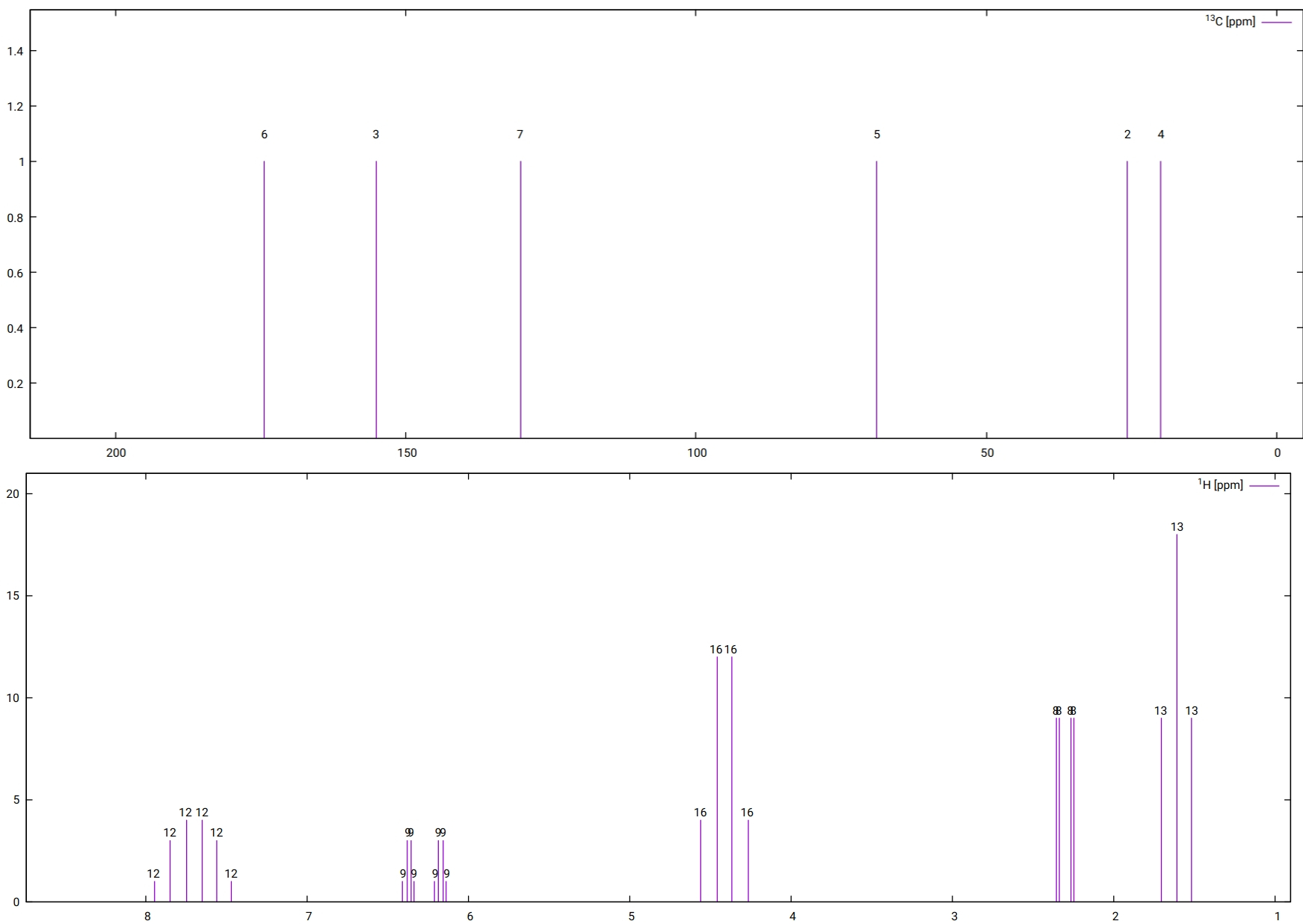
Fig. 6.54 Simulated \(^13C\) (top) and 1H (bottom) NMR spectra. Note that as only HH couplings have been computed, the spectra do not include any CH couplings and the carbon spectrum is also uncoupled.

This makes comparison to experiment and assessment of the computed parameters much easier, however, it is not as advanced as other codes and does not, for example, take conformational degrees of freedom etc. into account. Note that the corresponding property files can also be modified to tinker with the computed shieldings and couplings.

6.12.8.2. Visualizing shielding tensors using orca_plot

For the visualization it is recommended to perform an ORCA NMR calculation such that the corresponding gbw and density files required by orca_plot are generted by using the !keepdens keyword along with !NMR. If orca_plot is called in the interactive mode by specifying orca_plot myjob.gbw -i (note that myjob.gbw, myjob.densities and myjob.property.txt have to be in this directory), then following 1 - type of plot and choosing 17 - shielding tensor, confirming the name of the property file and then choosing 11 - Generate the plot will generate a .cube file with shielding tensors depicted as ellipsoids at the corrsponding nuclei. These can be plotted for example using Avogadro, isosurface values of around 1.0 and somewhat denser grids for the cube file (like 100x100x100) are recommended. A typical plot for CF\(_3\)SCH\(_3\) generated with Avogadro looks like this [6]:

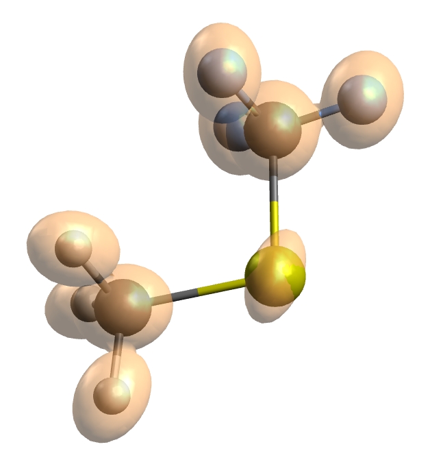
Fig. 6.55 The shielding tensors of each atom in CF3SCH3 have been plotted as ellipsoids (a,b and c axis equivalent to the normalized principle axes of the shielding tensors) at the given nuclei.

6.12.9. Hyperfine and Quadrupole Couplings

Hyperfine and quadrupole couplings can be obtained from the EPR/NMR module of ORCA. Since there may be several nuclei that you might be interested in the input is relatively sophisticated.

An example how to calculate the hyperfine and field gradient tensors for the CN radical is given below:

! PBE0 def2-MSVP TightSCF
* int 0 2
   C  0  0  0  0     0  0
   N  1  0  0  1.170 0  0
*
%eprnmr  Nuclei = all C { aiso, adip }
         Nuclei = 2 { aiso, adip, fgrad }
         end

In this example the hyperfine tensor is calculated for all carbon atoms and atom 2, which is nitrogen in this case.

Note

• counting of atom numbers starts from 1

• All nuclei mentioned in one line will be assigned the same isotopic mass, i.e. if several nuclei are calculated, there has to be a new line for each of them.

• You have to specify the Nuclei statement after the definition of the atomic coordinates or the program will not figure out what is meant by “all”.

The output looks like the following. It contains detailed information about the individual contributions to the hyperfine couplings, its orientation, its eigenvalues, the isotropic part and (if requested) also the quadrupole coupling tensor.

-----------------------------------------
ELECTRIC AND MAGNETIC HYPERFINE STRUCTURE
-----------------------------------------

 -----------------------------------------------------------
 Nucleus   0C : A:ISTP=   13 I=  0.5 P=134.1903 MHz/au**3
                Q:ISTP=   13 I=  0.5 Q=  0.0000 barn
 -----------------------------------------------------------
 Raw HFC matrix (all values in MHz):
 -----------------------------------
               695.8952               0.0000              -0.0000
                 0.0000             543.0617              -0.0000
                -0.0000              -0.0000             543.0617

 A(FC)         594.0062             594.0062             594.0062
 A(SD)         -50.9445             -50.9445             101.8890
             ----------           ----------           ----------
 A(Tot)        543.0617             543.0617             695.8952    A(iso)=  594.0062
 Orientation:
  X           0.0000000            0.0000000           -1.0000000
  Y          -0.8111216           -0.5848776           -0.0000000
  Z          -0.5848776            0.8111216            0.0000000

Notes:  (1) The A matrix conforms to the "SAI" spin Hamiltonian convention.
        (2) Tensor is right-handed.

 -----------------------------------------------------------
 Nucleus   1N : A:ISTP=   14 I=  1.0 P= 38.5677 MHz/au**3
                Q:ISTP=   14 I=  1.0 Q=  0.0204 barn
 -----------------------------------------------------------
 Raw HFC matrix (all values in MHz):
 -----------------------------------
                13.2095              -0.0000               0.0000
                -0.0000             -45.6036              -0.0000
                 0.0000              -0.0000             -45.6036

 A(FC)         -25.9993             -25.9993             -25.9993
 A(SD)          39.2088             -19.6044             -19.6044
             ----------           ----------           ----------
 A(Tot)         13.2095             -45.6036             -45.6036    A(iso)=  -25.9993
 Orientation:
  X           1.0000000            0.0000000           -0.0000000
  Y          -0.0000000            0.9996462            0.0265986
  Z           0.0000000           -0.0265986            0.9996462

Notes:  (1) The A matrix conforms to the "SAI" spin Hamiltonian convention.
        (2) Tensor is right-handed.

 Raw EFG matrix (all values in a.u.**-3):
 -----------------------------------
            -0.1832      -0.0000       0.0000
            -0.0000       0.0916       0.0000
             0.0000       0.0000       0.0916

 V(El)       0.6468       0.6468      -1.2935
 V(Nuc)     -0.5551      -0.5551       1.1103
         ----------   ----------   ----------
 V(Tot)      0.0916       0.0916      -0.1832
 Orientation:
  X      -0.0000003    0.0000002    1.0000000
  Y       0.9878165    0.1556229    0.0000003
  Z      -0.1556229    0.9878165   -0.0000002

Note: Tensor is right-handed


 Quadrupole tensor eigenvalues (in MHz;Q= 0.0204 I=  1.0)
  e**2qQ            =    -0.880 MHz
  e**2qQ/(4I*(2I-1))=    -0.220 MHz
  eta               =     0.000
  NOTE: the diagonal representation of the SH term I*Q*I = e**2qQ/(4I(2I-1))*[-(1-eta),-(1+eta),2]

Another important point to consider for hyperfine calculations concerns the choice of basis sets. You should normally use basis sets that have more flexibility in the core region. In the present example a double-zeta basis set was used. For accurate calculations this is not sufficient. There are several dedicated basis set for hyperfine calculations:

• EPR-II basis of Barone and co-workers: It is only available for a few light atoms (H, B, C, N, O, F) and is essentially of double-zeta plus polarization quality with added flexibility in the core region, which should give reasonable results.

• IGLO-II and IGLO-III bases of Kutzelnigg and co-workers: They are fairly accurate but also only available for some first and second row elements.

• CP basis: They are accurate for first row transition metals as well.

• uncontracted Partridge basis: They are general purpose HF-limit basis sets and will probably be too expensive for routine use, but are very useful for calibration purposes.

For other elements ORCA does not yet have dedicated default basis sets for this situation it is very likely that you have to tailor the basis set to your needs. If you use the statement Print[p_basis] 2 in the %output block (or PrintBasis in the simple input line) the program will print the actual basis set in input format (for the basis block). You can then add or remove primitives, uncontract core bases etc. For example, here is a printout of the carbon basis DZP in input format:

# Basis set for element : C
  NewGTO 6
  s 5
   1  3623.8613000000      0.0022633312
   2   544.0462100000      0.0173452633
   3   123.7433800000      0.0860412011
   4    34.7632090000      0.3022227208
   5    10.9333330000      0.6898436475
  s 1
   1     3.5744765000      1.0000000000
  s 1
    1    0.5748324500      1.0000000000
  s 1
    1    0.1730364000      1.0000000000
  p 3
    1    9.4432819000      0.0570590790
    2    2.0017986000      0.3134587330
    3    0.5462971800      0.7599881644
  p 1
    1    0.1520268400      1.0000000000
  d 1
    1    0.8000000000      1.0000000000
  end;

The “s 5”, for example, stands for the angular momentum and the number of primitives in the first basis function. Then there follow five lines that have the number of the primitive, the exponent and the contraction coefficient (unnormalized) in it. Remember also that when you add very steep functions you must increase the size of the integration grid if you do DFT calculations! If you do not do that your results will be inaccurate. You can increase the radial grid size by using IntAcc in the Method block or for individual atoms (section Other details and options explains how to do this in detail). In the present example the changes caused by larger basis sets in the core region and more accurate integration are relatively modest – on the order of 3%, which is, however, still significant if you are a little puristic.

The program can also calculate the spin-orbit coupling contribution to the hyperfine coupling tensor as described in section EPR and NMR properties.To extract the A tensor from a oligonuclear transition metal complex, the A(iso) value in the output is to be processed according to the method described in ref. [644].

For the calculation of HFCCs using DLPNO-CCSD it is recommended to use the tailored truncation settings !DLPNO-HFC1 or !DLPNO-HFC2 in the simple keyword line which correspond to the “Default1” and “Default2” setting in Ref. [742].

If also EPR g-tensor or D-tensor calculations (see next section) are carried out in the same job, ORCA automatically prints the orientation between the hyperfine/quadrupole couplings and the molecular g- or D-tensor. For more information on this see section orca_euler.

6.12.10. The EPR g-Tensor and the Zero-Field Splitting Tensor

The EPR g-tensor is a property that can be well calculated at the SCF level with ORCA through solution of the coupled-perturbed (CP-)SCF equations (see CP-SCF Options) and at the CASSCF level via the CP-CASSCF equations (see CASSCF Linear Response). As an example, consider the following simple g-tensor job:

! BP86 Def2-SVP TightSCF g-tensor SOMF(1X)
* int 1 2
   O  0  0  0  0      0  0
   H  1  0  0  1.1056 0  0
   H  1  2  0  1.1056 109.62 0
*

The simplest way is to call the g-tensor property in the simple input line as shown above, but it can also be specified in the %eprnmr block with gtensor true. Starting from ORCA 5.0 the default treatment of the gauge is the GIAO approach, but this can be modified by the keyword ori. Other options are defined in section EPR and NMR properties. SOMF(1X) defines the chosen spin-orbit coupling (SOC) operator. The details of the SOC operator are defined in section The Spin-Orbit Coupling Operator. Other choices and additional variables exist and can be set as explained in detail in section The Spin-Orbit Coupling Operator.

The output looks like the following. It contains information on the contributions to the g-tensor (relativistic mass correction, diamagnetic spin-orbit term (= gauge-correction), paramagnetic spin-orbit term (= OZ/SOC)), the isotropic g-value and the orientation of the total tensor.

-------------------
ELECTRONIC G-MATRIX
-------------------

The g-matrix:
              2.0104321   -0.0031354   -0.0000000
             -0.0031354    2.0081968   -0.0000000
             -0.0000000   -0.0000000    2.0021275

Breakdown of the contributions
 gel          2.0023193    2.0023193    2.0023193
 gRMC        -0.0003174   -0.0003174   -0.0003174
 gDSO(tot)    0.0000808    0.0001539    0.0001515
 gPSO(tot)    0.0000449    0.0038301    0.0104898
             ----------   ----------   ----------
 g(tot)       2.0021275    2.0059858    2.0126431 iso=  2.0069188
 Delta-g     -0.0001917    0.0036665    0.0103238 iso=  0.0045995

 Orientation:
  X           0.0000000    0.5762906   -0.8172448
  Y           0.0000000    0.8172448    0.5762906
  Z           1.0000000   -0.0000000    0.0000000

G-tensor calculations using GIAOs are now available at SCF and the RI-MP2 level. Note that GIAOs are NOT currently available with CASSCF linear response and a gauge origin must be provided in the %eprnmr block (see CASSCF Linear Response). GIAOs for CASSCF response are coming soon to ORCA!

The GIAO one-electron integrals are done analytically by default whereas the treatment of the GIAO two-electron integrals is chosen to be same as for the SCF. The available options which can be set with giao_1el / giao_2el in the %eprnmr block can be found in section EPR and NMR properties.

Concerning the computational time, for small systems, e.g. phenyl radical (41 electrons), the rijk-approximation is good to use for the SCF-procedures as well as the GIAO two-electron integrals. Going to larger systems, e.g. chlorophyll radical (473 electrons), the rijcosx-approximation reduces the computational time enormously. While the new default grid settings in ORCA 5.0 (defgrid2) should be sufficient in most cases, certain cases might need the use of defgrid3. The output looks just the same as for the case without GIAOs, but with additional information on the GIAO-parts.

If the total spin of the system is \(S\) >1/2 then the zero-field-splitting tensor can also be calculated and printed. For example consider the following job on a hypothetical Mn(III)-complex.

! BP86 def2-SVP SOMF(1X)

%eprnmr DTensor  ssandso  
        DSOC     cp  # qro, pk, cvw
        DSS      uno # direct
        end

* int  1 5
Mn 0 0 0  0 0 0
 O 1 0 0  2.05   0   0
 O 1 2 0  2.05  90   0
 O 1 2 3  2.05  90 180
 O 1 2 3  2.05 180   0
 F 1 2 3  1.90  90  90
 F 1 2 3  1.90  90 270
 H 2 1 6  1.00 127   0
 H 2 1 6  1.00 127 180
 H 3 1 6  1.00 127   0
 H 3 1 6  1.00 127 180
 H 4 1 6  1.00 127   0
 H 4 1 6  1.00 127 180
 H 5 1 6  1.00 127   0
 H 5 1 6  1.00 127 180
*

The output documents the individual contributions to the D-tensor which also contains (unlike the g-tensor) contributions from spin-flip terms.

Some explanation must be provided:

• The present implementation in ORCA is valid for HF, DFT and hybrid DFT.

• There are four different variants of the SOC-contribution, which shows that this is a difficult property. We will briefly discuss the various choices.

• The QRO method is fully documented[611] and is based on a theory developed earlier.[621] The QRO method is reasonable but somewhat simplistic and is superseded by the CP method described below.

• The Pederson-Khanna model was brought forward in 1999 from qualitative reasoning.[656] It also contains incorrect prefactors for the spin-flip terms. We have nevertheless implemented the method for comparison. In the original form it is only valid for local functionals. In ORCA it is extended to hybrid functionals and HF.

• The coupled-perturbed method is a generalization of the DFT method for ZFSs; it uses revised prefactors for the spin-flip terms and solves a set of coupled-perturbed equations for the SOC perturbation. Therefore it is valid for hybrid functionals. It has been described in detail.[613]

• The DSS part is an expectation value that involves the spin density of the system. In detailed calibration work[799] it was found that the spin-unrestricted DFT methods behave somewhat erratically and that much more accurate values were obtained from open-shell spin-restricted DFT. Therefore the “UNO” option allows the calculation of the SS term with a restricted spin density obtained from the singly occupied unrestricted natural orbitals.

• The DSS part contains an erratic self-interaction term for UKS/UHF wavefunction and canonical orbitals. Thus, UNO is recommended for these types of calculations.[723] If the option DIRECT is used nevertheless, ORCA will print a warning in the respective part of the output.

• In case that D-tensor is calculated using the correlated wave function methods such as (DLPNO-/LPNO-)CCSD, one should not use DSS=UNO option.

More information about the D-tensor can be found in section Zero-Field-Splitting.

6.12.11. Mössbauer Parameters

\(^{57}\)Fe Mössbauer spectroscopy probes the transitions of the nucleus between the \(I = \frac{1}{2}\) ground state and the \(I = \frac{3}{2}\) excited state at 14.4 keV above the ground state. The important features of the Mössbauer spectrum are the isomer shift (\(\delta\)) and the quadrupole splitting (\(\Delta E_\mathrm{Q}\)). An idealized spectrum is shown in Fig. 6.56.

Fig. 6.56 An idealized Mössbauer spectrum showing both the isomer shift, \(\delta\), and the quadrupole splitting, \(\Delta E_\mathrm{Q}\).

The isomer shift measures the shift in the energy of the \(\gamma\)-ray absorption relative to a standard, usually Fe foil. The isomer shift is sensitive to the electron density at the nucleus, and indirectly probes changes in the bonding of the valence orbitals due to variations in covalency and 3d shielding. Thus, it can be used to probe oxidation and spin states, and the coordination environment of the iron.

The quadrupole splitting arises from the interaction of the nuclear quadrupole moment of the excited state with the electric field gradient at the nucleus. The former is related to the non-spherical charge distribution in the excited state. As such it is extremely sensitive to the coordination environment and the geometry of the complex.

Both the isomer shift and quadrupole splitting can be successfully predicted using DFT methods. The isomer shift is directly related to the s electron density at the nucleus and can be calculated using the formula

(6.14)\[\delta = \alpha (\rho_0 - C) + \beta \]

where \(\alpha\) is a constant that depends on the change in the distribution of the nuclear charge upon absorption, and \(\rho_0\) is the electron density at the nucleus [608]. The constants \(\alpha\) and \(\beta\) are usually determined via linear regression analysis of the experimental isomer shifts versus the theoretically calculated electron density for a series of iron compounds with various oxidation and spin states. Since the electron density depends on the functional and basis set employed, fitting must be carried out for each combination used. A compilation of calibration constants (\(\alpha\), \(\beta\) and \(C\)) for various methods was assembled.[707] Usually an accuracy of better than 0.10 mm s\(^{-1}\) can be achieved for DFT with reasonably sized basis sets.

The quadrupole splitting is proportional to the largest component of the electric field gradient (EFG) tensor at the iron nucleus and can be calculated using the formula:

(6.15)\[\Delta E_\mathrm{Q} = \frac{1}{2}eQV_{zz} \left( 1+\frac{\eta^2}{3} \right)^{\frac{1}{2} } \]

where \(e\) is the electrical charge of an electron and \(Q\) is the nuclear quadrupole moment of Fe (approximately 0.16 barns). \(V_{xx}\), \(V_{yy}\) and \(V_{zz}\) are the electric field gradient tensors and \(\eta\), defined as

(6.16)\[\eta = \left| \frac{V_{xx} - V_{yy} }{V_{zz} } \right|\]

is the asymmetry parameter in a coordinate system chosen such that \(|V_{zz}| \geq |V_{yy}| \geq |V_{xx}|\).

An example of how to calculate the electron density and quadrupole splitting of an iron center is as follows:

%eprnmr
  nuclei = all Fe {fgrad, rho}
end

If the core properties basis set CP(PPP) is employed, one might have to increase the radial integration accuracy for the iron atom. From ORCA 5.0 this is considered during grid construction and the defaults should work very well. However for very problematic cases it can be increased by controlling the SPECIALGRIDINTACC flag under %METHOD (see Sec. Other details and options for details).

The output file should contain the following lines, where you obtain the calculated quadrupole splitting directly and the RHO(0) value (the electron density at the iron nucleus). To obtain the isomer shift one has to insert the RHO(0) value into the appropriate linear equation (Eq. (6.14)).

Moessbauer quadrupole splitting parameter (proper coordinate system)
e**2qQ  = -0.406 MHz = -0.035 mm/s
eta     = 0.871
Delta-EQ=(1/2{e**2qQ}*sqrt(1+1/3*eta**2) = -0.227 MHz = -0.020 mm/s
RHO(0)=  11581.352209571 a.u.**-3   # the electron density at the Fe nucleus.

Note

• Following the same procedure, Mössbauer parameters can be computed with the CASSCF wavefunction. In case of a state-averaged CASSCF calculation, the averaged density is used in the subsequent Mössbauer calculation.

6.12.12. Broken-Symmetry Wavefunctions and Exchange Couplings

A popular way to estimate the phenomenological parameter \(J_{\mathrm{AB} }\) that enters the Heisenberg–Dirac–van Vleck Hamiltonian which parameterizes the interaction between two spin systems is the “broken-symmetry” formalism. The phenomenological Hamiltonian is:

(6.17)\[H_{\mathrm{HDvV} } = -2J_{\mathrm{AB} } \vec{{S} }_{\mathrm{A} } \vec{{S} }_{\mathrm{B} } \]

It is easy to show that such a Hamiltonian leads to a “ladder” of spin states from \(S=S_{\mathrm{A} } + S_{\mathrm{B} }\) down to \(S=\left|{ S_{\mathrm{A} } - S_{\mathrm{B} }} \right|\). If the parameter \(J_{\mathrm{AB} }\) is positive the systems “A” and “B” are said to be ferromagnetically coupled because the highest spin-state is lowest in energy while in the case that \(J_{\mathrm{AB} }\) is negative the coupling is antiferromagnetic and the lowest spin state is lowest in energy.

In the broken symmetry formalism one tries to obtain a wavefunction that breaks spatial (and spin) symmetry. It may be thought of as a “poor man’s MC-SCF” that simulates a multideterminantal character within a single determinant framework. Much could be said about the theoretical advantages, disadvantages, problems and assumptions that underly this approach. Here, we only want to show how this formalism is applied within ORCA.

For \(N_{\mathrm{A} }\) unpaired electrons localized on “site A” and \(N_{\mathrm{B} }\) unpaired electrons localized on a “site B” one can calculate the parameter \(J_{\mathrm{AB} }\) from two separate spin-unrestricted SCF calculations: (a) the calculation for the high-spin state with \(S=\frac{\left({ N_{\mathrm{A} } + N_{\mathrm{B} }} \right)}{2}\) and (b) the “broken symmetry” calculation with \(M_{S} = \frac{\left({ N_{\mathrm{A} } -N_{\mathrm{B} } } \right)}{2}\) that features \(N_{\mathrm{A} }\) spin-up electrons that are quasi-localized on “site A” and \(N_{\mathrm{B} }\) spin-down electrons that are quasi-localized on “site B”. Several formalisms exist to extract \(J_{\mathrm{AB} }\): [91, 303, 636, 637, 808, 897].

(6.18)\[J_{\mathrm{AB} } = - \frac{\left({ E_{\mathrm{HS} } -E_{\mathrm{BS} } } \right)}{\left({ S_{\mathrm{A} } +S_{\mathrm{B} } } \right)^{2} } \]

(6.19)\[J_{\mathrm{AB} } = -\frac{\left({ E_{\mathrm{HS} } -E_{\mathrm{BS} } } \right)}{\left({ S_{\mathrm{A} } +S_{\mathrm{B} } } \right)\left({ S_{\mathrm{A} } +S_{\mathrm{B} } +1} \right)} \]

(6.20)\[J_{\mathrm{AB} } =-\frac{\left({ E_{\mathrm{HS} } -E_{\mathrm{BS} } } \right)}{\left\langle { S^{2} } \right\rangle_{\mathrm{HS} } -\left\langle { S^{2} } \right\rangle_{\mathrm{BS} } } \]

We prefer the last definition (Eq. (6.20)) because it is approximately valid over the whole coupling strength regime while the first equation implies the weak coupling limit and the second the strong coupling limit.

In order to apply the broken symmetry formalism use:

%scf BrokenSym NA,NB
     end

The program will then go through a number of steps. Essentially it computes an energy and wavefunction for the high-spin state, localizes the orbitals and reconverges to the broken symmetry state.

Caution

Make sure that in your input coordinates “site A” is the site that contains the larger number of unpaired electrons!

Most often the formalism is applied to spin coupling in transition metal complexes or metal-radical coupling or to the calculation of the potential energy surfaces in the case of homolytic bond cleavage. In general, hybrid DFT methods appear to give reasonable semiquantitative results for the experimentally observed splittings.

As an example consider the following simple calculation of the singlet–triplet splitting in a stretched Li\(_{2}\) molecule:

#
# Example of a broken symmetry calculation
#
! B3LYP DEF2-SVP TightSCF
%scf BrokenSym 1,1
     end
* xyz 0 3
  Li  0  0  0
  Li  0  0  4
*

There is a second mechanism for generating broken-symmetry solutions in ORCA. This mechanism uses the individual spin densities and is invoked with the keywords FlipSpin and FinalMs. The strategy is to exchange the \(\alpha\) and \(\beta\) spin blocks of the density on certain user-defined centers after converging the high-spin wavefunction. With this method arbitrary spin topologies should be accessible. The use is simple:

#
# Example of a broken symmetry calculation using the "FlipSpin" feature
#
! B3LYP DEF2-SVP TightSCF
%scf 
     FlipSpin 1
       # Flip spin is a vector and you can give a list of atoms
       # on which you want to have the spin flipped. For example
       #  FlipSpin 17,38,56  
       # REMEMBER: counting starts at atom 0!
     FinalMs  0
       # The desired Ms value of the broken symmetry determinant.
       # This value MUST be given since the program cannot determine it by itself.
     end
* xyz 0 3
  Li  0  0  0
  Li  0  0  4
*

Finally, you may attempt to break the symmetry by using the SCF stability analysis feature (see Section SCF Stability Analysis). The ground spin state can be obtained by diagonalizing the above spin Hamiltonian through ORCA-ECA utility (see orca_eca).

6.12.12.1. Approximate Spin Projection Method

The approximate spin projection (AP) method, proposed by Yamaguchi and co-workers, is a technique to remove the spin contamination from exchange coupling constants.[737, 896, 897] In this scheme, the energy of a system is given by

(6.21)\[ E_{\mathrm{AP} }=\alpha E_{\mathrm{BS} }-\left(\alpha - 1\right)E_{\mathrm{HS} } \]

The parameter \(\alpha\) is calculated as

(6.22)\[ \alpha=\frac{S^{\mathrm{HS} }\left(S^{\mathrm{HS} }+1\right) - S_Z^{\mathrm{BS} }\left(S_Z^{\mathrm{BS} }+1\right)}{\langle\hat{\mathbf{S} }^2\rangle^{\mathrm{HS} }-\langle\hat{\mathbf{S} }^2\rangle^{\mathrm{BS} }} \]

Here, \(S_Z^{\mathrm{BS} }\) is the \(z\)-component of the total spin for the BS state (\(S_Z^{\mathrm{BS} }=(N_{\alpha}-N_{\beta})/2\)). Alternatively, one can adopt Noodleman’s scheme,[637] where \(\alpha\) is calculated as follows

(6.23)\[ \alpha=\frac{S^{\mathrm{HS} }\left(S^{\mathrm{HS} }+1\right) - S_Z^{\mathrm{BS} }\left(S_Z^{\mathrm{BS} }+1\right)}{\left(S^{\mathrm{HS} }\right)^2} \]

or Ruiz’s scheme,[733] with \(\alpha\) equal to

(6.24)\[ \alpha=\frac{S^{\mathrm{HS} }\left(S^{\mathrm{HS} }+1\right) - S_Z^{\mathrm{BS} }\left(S_Z^{\mathrm{BS} }+1\right)}{S^{\mathrm{HS} }\left(S^{\mathrm{HS} }+1\right)} \]

The AP method is requested via the tag APMethod in the %scf block:

%scf BrokenSym NA,NB
     APMethod 3  # 1 = Noodleman
                 # 2 = Ruiz
                 # 3 = Yamaguchi
end

The default is APMethod 0, which corresponds to a normal BS calculation. Yamaguchi’s AP method is available for single point energy calculations and geometry optimizations. If we run a geometry optimization in the context of Yamaguchi’s AP method, then, the gradient of equation (6.21) w.r.t a nuclear displacement \(X\) reads as

(6.25)\[ \frac{\partial E_{\mathrm{AP} }}{\partial X}=\alpha\frac{\partial E_{\mathrm{BS} }}{\partial X}-\left(\alpha-1\right)\frac{\partial E_{\mathrm{HS} }}{\partial X}+\frac{\partial\alpha}{\partial X}\left(E_{\mathrm{BS} } - E_{\mathrm{HS} }\right) \]

The last term contains the derivative \(\frac{\partial\alpha}{\partial X}\). ORCA uses the formalism proposed by Saito and Thiel, which involves solving the CP-SCF equations in each geometry optimization cycle.[738] The cost of such a calculation is higher than using Noodleman’s or Ruiz’s schemes, where \(\frac{\partial\alpha}{\partial X}=0\).

6.13. Local Energy Decomposition

“Local Energy Decomposition” (LED) analysis[33, 105, 767] is a tool for obtaining insights into the nature of intermolecular interactions by decomposing the DLPNO-CCSD(T) energy into physically meaningful contributions. For instance, this approach can be used to decompose the DLPNO-CCSD(T) interaction energy between a pair of interacting fragments, as detailed in Section Local Energy Decomposition. A useful comparison of this scheme with alternative ways of decomposing interaction energies is reported in Ref. [27, 28, 29].

6.13.1. Closed shell LED

All that is required to obtain this decomposition in ORCA is to define the fragments and specify the !LED keyword in the simple input line.

LED decomposes separately the reference (Hartree-Fock) and correlation parts of the DLPNO-CCSD(T) energy. By default, the decomposition of the reference energy makes use of the RI-JK approximation. An RIJCOSX variant, which is much more efficient and has a much more favorable scaling for large systems, is also available, as detailed in section Additional Features, Defaults and List of Keywords, and in [27].

Note that, for weakly interacting systems, TightPNO settings are typically recommended. As an example, the interaction of H\(_2\)O with the carbene CH\(_2\) at the PBE0-D3/def2-TZVP-optimized geometry can be analyzed within the LED framework using the following input file:

! dlpno-ccsd(t) cc-pvdz cc-pvdz/c cc-pvtz/jk rijk verytightscf TightPNO LED

*xyz 0 1
  C(1)      0.16044643459993      0.10093183177121      0.22603351276210
  H(1)      1.04516129053973     -0.06834886965353     -0.41865951747519
  H(1)     -0.12579332868173      1.14737893892114      0.00305818518771
  O(2)     -1.48285705560792     -1.31933824653169      2.29891474420047
  H(2)     -0.91417368674145     -0.93085192992263      1.60917234463506
  H(2)     -1.15648922489703     -2.21246650333085      2.42094328175662
*

The corresponding output file is reported below. The DLPNO-CCSD(T) energy components are printed out in different parts of the output as follows:

E(0)                                       ...   -114.913309038
E(CORR)(corrected)                         ...     -0.350582526 
Triples Correction (T)                     ...     -0.006098691
E(CCSD(T))                                 ...   -115.269990255

At the beginning of the LED part of the output, information on the fragments and the assignment of localized MOs to fragments are provided.

 ===========================================================
         LOCAL ENERGY DECOMPOSITION FOR DLPNO-CC METHODS
 ===========================================================

Maximum Iterations for the Localization .. 600
Tolerance for the Localization          ..  1.00e-06
Number of fragments = 2
Fragment  1:  0 1 2
Fragment  2:  3 4 5

Populations of internal orbitals onto Fragments:
   0:      1.000    0.000  assigned to fragment   1
   1:      0.000    1.000  assigned to fragment   2
   2:      1.022    0.008  assigned to fragment   1
   3:      0.001    0.999  assigned to fragment   2
   4:      0.001    0.999  assigned to fragment   2
   5:      1.018    0.000  assigned to fragment   1
   6:      1.019    0.000  assigned to fragment   1
   7:      0.006    1.013  assigned to fragment   2
   8:      0.000    1.016  assigned to fragment   2

The decomposition of the Hatree-Fock energy into intra- and inter-fragment contributions follows. It is based on the localization of the occupied orbitals.

----------------------------------------
REFERENCE ENERGY E(0) DECOMPOSITION (Eh)
----------------------------------------

Nuclear repulsion     =        28.952049689006
One electron energy   =      -214.430545074583 (T=      114.825132245389, V=     -329.255677319972)
Two electron energy   =        70.565186347093 (J=       71.658914661909, K=       -1.093728314816)
                        ----------------------
Total energy          =      -114.913309038483
Consistency check     =      -114.913309038483 (sum of intra- and inter-fragment energies)

Kinetic energy        =       114.825132245389
Potential energy      =      -229.738441283873
                        ----------------------
Virial ratio          =         2.000767922417

-------------------------------------------
INTRA-FRAGMENT REF. ENERGY FOR FRAGMENT   1
-------------------------------------------

Nuclear repulsion     =         6.037208782874
One electron energy   =       -63.553431032444 (T=       38.870491681225, V=     -102.423922713669)
Two electron energy   =        18.675214766985 (J=       18.935443192480, K=       -0.260228425495)
                        ----------------------
Total energy          =       -38.841007482585

Kinetic energy        =        38.870491681225
Potential energy      =       -77.711499163811
                        ----------------------
Virial ratio          =         1.999241476056


-------------------------------------------
INTRA-FRAGMENT REF. ENERGY FOR FRAGMENT   2
-------------------------------------------

Nuclear repulsion     =         9.103529882464
One electron energy   =      -123.025684625357 (T=       75.954640564164, V=     -198.980325189521)
Two electron energy   =        37.916781954190 (J=       38.739989208810, K=       -0.823207254620)
                        ----------------------
Total energy          =       -76.005372788703

Kinetic energy        =        75.954640564164
Potential energy      =      -151.960013352867
                        ----------------------
Virial ratio          =         2.000667927913


----------------------------------------------------
INTER-FRAGMENT REF. ENERGY FOR FRAGMENTs   2 AND   1
----------------------------------------------------

Nuclear repulsion     =        13.811311023669
Nuclear attraction    =       -27.851429416782
Coulomb repulsion     =        13.983482260618
                        ----------------------
Sum of electrostatics =        -0.056636132494 (  -35.540 kcal/mol)

Two electron exchange =        -0.010292634701 (   -6.459 kcal/mol)
                        ----------------------
Total REF. interaction =       -0.066928767195 (  -41.998 kcal/mol)



Sum of INTRA-fragment REF. energies  =      -114.846380271288
Sum of INTER-fragment REF. energies  =        -0.066928767195
                                      ---------------------
Total REF. energy                    =      -114.913309038483

Afterwards, a first decomposition of the correlation energy is carried out. The different energy contributions to the correlation energy (strong pairs, weak pairs and triples correction) are decomposed into intra- and inter-fragment contributions. This decomposition is carried out based on the localization of the occupied orbitals.

--------------------------------
CORRELATION ENERGY DECOMPOSITION
--------------------------------


--------------------------------------------------
INTER- vs INTRA-FRAGMENT CORRELATION ENERGIES (Eh)
--------------------------------------------------

                                   Fragment   1            Fragment   2
                         ----------------------  ----------------------
Intra strong pairs              -0.136594658271        -0.209970193798  sum=       -0.346564852069
Intra triples                   -0.002692277706        -0.002842791265  sum=       -0.005535068971
Intra weak pairs                -0.000001573694        -0.000002311734  sum=       -0.000003885429
Singles contribution             0.000000000611         0.000000001058  sum=        0.000000001669
                         ----------------------  ----------------------
                                -0.139288509061        -0.212815295738  sum=       -0.352103804799


Interaction correlation for Fragments   2 and   1:
--------------------------------------------------
Inter strong pairs               -0.003998018810 (   -2.509 kcal/mol)
Inter triples                    -0.000563621667 (   -0.354 kcal/mol)
Inter weak pairs                 -0.000015771468 (   -0.010 kcal/mol)
                          ----------------------
Total interaction                -0.004577411945 (   -2.872 kcal/mol)



Sum of INTRA-fragment correlation energies  =        -0.352103804799
Sum of INTER-fragment correlation energies  =        -0.004577411945
                                              ---------------------
Total correlation energy                    =        -0.356681216744

Afterwards, a summary with the decomposition of the total energy (reference energy + correlation) into intra- and inter-fragment contributions is printed.

--------------------------------------------
INTER- vs INTRA-FRAGMENT TOTAL ENERGIES (Eh)
--------------------------------------------

                                   Fragment   1            Fragment   2
                         ----------------------  ----------------------
Intra REF. energy              -38.841007482585       -76.005372788703  sum=     -114.846380271288
Intra Correlation energy        -0.139288509061        -0.212815295738  sum=       -0.352103804799
                         ----------------------  ----------------------
                               -38.980295991646       -76.218188084441  sum=     -115.198484076087


Interaction of Fragments   2 and   1:
-------------------------------------
Interfragment reference          -0.066928767195 (  -41.998 kcal/mol)
Interfragment correlation        -0.004577411945 (   -2.872 kcal/mol)
                          ----------------------
Total interaction                -0.071506179140 (  -44.871 kcal/mol)


Sum of INTRA-fragment total energies        =      -115.198484076087
Sum of INTER-fragment total energies        =        -0.071506179140
                                              ---------------------
Total energy                                =      -115.269990255228

Hence, the decomposition reported above allows one to decompose all the components of the DLPNO-CCSD(T) energy into intrafragment and interfragment contributions simply based on the localization of the occupied orbitals. In order to convert the intra-fragment energy components into contributions to the binding energy, single point energy calculations must be carried out on the isolated monomers, frozen in the geometry they have in the adduct, and the corresponding terms must be subtracted. Note that one can also include the geometrical deformation energy (also called “strain”) by simply computing the energy of the geometrically relaxed fragments (see Section Local Energy Decomposition for further information).

For the DLPNO-CCSD strong pairs, which typically dominate the correlation energy, a more sophisticated decomposition, based on the localization of both occupied orbitals and PNOs, is also carried out and printed. Accordingly, the correlation energy from the strong pairs is divided into intra-fragment, dispersion and charge transfer components. Note that, due to the charge transfer excitations, the resulting intra-fragment contributions (shown below) differ from the ones obtained above.

---------------------------------------------
DECOMPOSITION OF CCSD STRONG PAIRS INTO
    DOUBLE EXCITATION TYPES (Eh)
---------------------------------------------

Foster-Boys localization is used for localizing PNOs

Intra fragment contributions:
INTRA Fragment 1                       -0.132849855
INTRA Fragment 2                       -0.209493798

Charge transfer contributions:
Charge Transfer 1 to 2                 -0.005725404
Charge Transfer 2 to 1                 -0.000899609

Dispersion contributions:
Dispersion  2,1                        -0.001594204

Singles contributions:
Singles energy                          0.000000002

More detailed information into the terms reported above can be found in Section Local Energy Decomposition and in Ref.[767] All the individual double excitations contributions constituting the terms reported above can be printed by specifying “printlevel 3” in the %mdci block. Finally, a summary with the most important terms of the DLPNO-CCSD energy, which are typically discussed in standard applications, is printed.

-------------------------------------------------
FINAL SUMMARY DLPNO-CCSD ENERGY DECOMPOSITION (Eh)
-------------------------------------------------

Intrafragment REF. energy:
Intra fragment   1 (REF.)              -38.841007483
Intra fragment   2 (REF.)              -76.005372789

Interaction of fragments  2 and  1:
Electrostatics (REF.)                  -0.056636132
Exchange (REF.)                        -0.010292635
Dispersion (strong pairs)              -0.001594204
Dispersion (weak pairs)                -0.000015771

Sum of non dispersive correlation terms:
Non dispersion (strong pairs)          -0.348968665
Non dispersion (weak pairs)            -0.000003885

Note that the “Non dispersion” terms include all the components of the correlation energy except London dispersion.[28, 106]. For the strong pairs, “Non dispersion” includes charge transfer, intrafragment double excitations and singles contributions. For the weak pairs, it corresponds to the intrafragment correlation contribution. In order to convert the non dispersion correlation components into contributions to the binding energy, single point energy calculations must be carried out on the isolated monomers.

6.13.2. Example: LED analysis of intermolecular interactions

The water-carbene example from the previous section will be used to demonstrate how to analyze intermolecular interactions between two fragments using the LED decomposition (note that all energies are given in a.u. if not denoted otherwise). As often done in practical applications, we will be using geometries optimized at the DFT (PBE0-D3/def2-TZVP) level of theory on which DLPNO-CCSD(T) (cc-pVDZ,TightPNO) single point energies are computed. Note that in practice, basis sets of triple-zeta quality or larger are recommended. In the first step, the geometries of the dimer, H\(_2\)O and CH\(_2\) are optimized and DLPNO-CCSD(T) energies are computed to yield \(E^{opt}_{dimer}\) and \(E^{opt}_{monomers}\). The input examples for the single-point DLPNO-CCSD(T) energies of the monomers at their optimized geometries and the necessary energies from the output files of these runs are as follows:

! dlpno-ccsd(t) cc-pvdz cc-pvdz/c cc-pvtz/jk rijk verytightscf TightPNO

# H2O optimized at the PBE0-D3/def2-TZVP level

*xyz 0 1
  O     -1.47291471015599     -1.29006364761118      2.29452038079177
  H     -0.88264582939506     -0.99404999457575      1.59835337186103
  H     -1.22136730983407     -2.20010680974562      2.46533021449572
*

E(0)                                       ...    -76.026656692
E(CORR)(corrected)                         ...     -0.211428886
Triples Correction (T)                     ...     -0.002932804
E(CCSD(T))                                 ...    -76.241018382

! dlpno-ccsd(t) cc-pvdz cc-pvdz/c cc-pvtz/jk rijk verytightscf TightPNO

# CH2 optimized at the PBE0-D3/def2-TZVP level 

*xyz 0 1
  C      0.16044643459993      0.10093183177121      0.22603351276210
  H      1.04516129053973     -0.06834886965353     -0.41865951747519
  H     -0.12579332868173      1.14737893892114      0.00305818518771
*

E(0)                                       ...    -38.881042677
E(CORR)(corrected)                         ...     -0.138447953
Triples Correction (T)                     ...     -0.002873032
E(CCSD(T))                                 ...    -39.022363662

Single-point DLPNO-CCSD(T) energies of the monomers at their in-adduct geometries are also necessary. The corresponding inputs and the necessary output parts for these calculations are as follows:

! dlpno-ccsd(t) cc-pvdz cc-pvdz/c cc-pvtz/jk rijk verytightscf TightPNO

# H2O at the CH2-H2O geometry optimized at the PBE0-D3/def2-TZVP level 

*xyz 0 1
  O     -1.48285705560792     -1.31933824653169      2.29891474420047
  H     -0.91417368674145     -0.93085192992263      1.60917234463506
  H     -1.15648922489703     -2.21246650333085      2.42094328175662

E(0)                                       ...    -76.026011663
E(CORR)(corrected)                         ...     -0.211931843
Triples Correction (T)                     ...     -0.002963338
E(CCSD(T))                                 ...    -76.240906844

! dlpno-ccsd(t) cc-pvdz cc-pvdz/c cc-pvtz/jk rijk verytightscf TightPNO

# CH2 at the CH2-H2O geometry optimized at the PBE0-D3/def2-TZVP level 

*xyz 0 1
  C      0.16044643459993      0.10093183177121      0.22603351276210
  H      1.04516129053973     -0.06834886965353     -0.41865951747519
  H     -0.12579332868173      1.14737893892114      0.00305818518771
*

E(0)                                       ...    -38.881085139
E(CORR)(corrected)                         ...     -0.138097323
Triples Correction (T)                     ...     -0.002869022
E(CCSD(T))                                 ...    -39.022051484

These energies are summarized in Table Table 6.9).

Table 6.9 Energies of the H\(_2\)O-CH\(_2\) example for illustrating how the different LED contributions are valuated. The superscript \(^{opt}\) denotes energies of optimized structures, \(^{fixed}\) denotes energies of isolated fragments in the dimer structure. In the last column the energy of the dimer is reported.

Energy [a.u.]	H\(_2O^{opt}\)	H\(_2O^{fixed}\)	CH\(_2^{opt}\)	CH\(_2^{fixed}\)	H\(_2\)O - CH\(_2\)
E\(_{HF}\)	-76.026656692	-76.026011663	-38.881042677	-38.881085139	-114.913309038
E\(_c\) CCSD	-0.211428886	-0.211931843	-0.138447953	-0.138097323	-0.350582526
E\(_c\) (T)	-0.002932804	-0.002963338	-0.002873032	-0.002869022	-0.006098691
E\(_{tot}\)	-76.241018382	-76.240906844	-39.022363662	-39.022051484	-115.269990255

Note that for this example, we do not include any BSSE correction. For this system we obtain a binding energy of

\[E_{int} = E^{opt}_{dimer} - E^{opt}_{monomers} = -115.269990255~ -~ (-76.241018382 -39.022363662) = -0.006608211\]

which is -4.147 kcal/mol.

The basic principles and the details of the LED are discussed in section Local Energy Decomposition. The first contribution to the binding energy is the energy penalty for the monomers to distort into the geometry of the dimer

\[\Delta E_{geo - prep}^{} = E^{fixed}_{monomers}-E^{opt}_{monomers}\]

(see in equation (7.408)). This contribution is computed as the difference of the DLPNO-CCSD(T) energy of the monomers in the structure of the dimer (\(E^{fixed}_{monomers}\)) and of the relaxed monomers (\(E^{opt}_{monomers}\)). The following energies are obtained:

\[\Delta E_{geo - prep}^{} = (-76.240906844+76.241018382) ~ + ~ (-39.022051484+39.022363662) = 0.000423716\]

which amounts to 0.266 kcal/mol. Typically, the triples correction is evaluated separately:

\[\Delta E^{C-(T) }_{int} = -0.006098691 - (-0.002963338 -0.002869022) = -0.000266331\]

This contributes -0.167 kcal/mol. The next terms in equation (7.408) concern the reference energy contributions. The first one is the electronic preparation in the reference, which is evaluated as the difference of the Intra REF. energy of the fragments (see previous section) and the reference energy of the separate molecules at the dimer geometry:

\[\Delta E_{el-prep}^{ref.}(H_2O) = -76.005372788703+76.026011663 = 0.020638874297\]

\[\Delta E_{el-prep}^{ref.}(CH_2) = -38.841007482585+38.881085139 = 0.040077656415\]

which amounts to 0.060716530712 a.u. or 38.100 kcal/mol. The next two contributions stem from the decomposition of the reference inter-fragment contributions \(E_{elstat}^{ref.} = -0.056636132\) (-35.540 kcal/mol) and \(E_{exch}^{ref.} = -0.010292635\) (-6.459 kcal/mol) and can be found in directly in the LED output (Electrostatics (REF.) and Exchange (REF.) ). The correlation energy also contains an electronic preparation contribution, but it is typically included in the correlation contribution \(\Delta E^{C-CCSD}_{non-dispersion}\). Adding the non-dispersive strong and weak pairs contributions from the LED output (Non dispersion (strong pairs) and Non dispersion (weak pairs) ) one obtains :

\[-0.348968665-0.000003885 = -0.34897255\]

from which we have to subtract the sum of the correlation contributions of the monomers at the dimer geometry

\[\Delta E^{C-CCSD}_{non-dispersion} = -0.34897255 - (-0.211931843-0.138097323) = 0.001056616\]

which is 0.663 kcal/mol. The dispersive contribution can be directly found in the LED output (Dispersion (strong pairs) and Dispersion (weak pairs) ) and amounts to \(E^{C-CCSD}_{dispersion} = -0.001609975\) which is -1.010 kcal/mol. So all terms that we have evaluated so far are:

\[\Delta E = \Delta E_{geo - prep}^{} + \Delta E_{el-prep}^{ref.} + E_{elstat}^{ref.} + E_{exch}^{ref.} + \Delta E^{C-CCSD}_{non-dispersion} + E^{C-CCSD}_{dispersion} + \Delta E^{C-(T) }_{int}\]

\(\Delta E\)	\(\Delta E_{geo-prep}\)	\(\Delta E_{el-prep}^{ref.}\)	\(E_{elstat}^{ref.}\)	\(E_{exch}^{ref.}\)	\(\Delta E^{C-CCSD}_{non-disp.}\)	\(E^{C-CCSD}_{disp.}\)	\(\Delta E^{C-(T)}_{int}\)
a.u.	0.000423716	0.060716530712	-0.056636132	-0.010292635	0.001056616	-0.001609975	-0.000266331
kcal/mol	0.266	38.100	-35.540	-6.459	0.663	-1.010	-0.167

which sum to the total binding energies of -0.006608211 a.u. or -4.147 kcal/mol that we have evaluated at the beginning of this section. A detailed discussion of the underlying physics and chemistry can be found in  [33].

6.13.3. Open shell LED

The decomposition of the DLPNO-CCSD(T) energy in the open shell case is carried out similarly to the closed shell case. [33] An example of input file is shown below.

! dlpno-ccsd(t) cc-pvdz cc-pvdz/c cc-pvtz/jk rijk verytightscf TightPNO LED

*xyz 0 3
C(1)      0.32786304018834      0.25137292674595      0.32985672433579
H(1)      0.78308855251826     -0.37244139824620     -0.42204823336026
H(1)     -0.19639272865450      1.19309490346756      0.33713773666060
O(2)     -1.47005964014997     -1.60804001777555      1.84974416203666
H(2)     -0.89305417808014     -1.00736849071095      1.35216686141176
H(2)     -1.02515061661047     -1.73931270222718      2.69260529998224
*

The corresponding output is entirely equivalent to the one just discussed for the closed shell case. However, the open shell variant of the LED scheme relies on a different implementation than the closed shell one. A few important differences exist between the two implementations, which are listed below.

• In the closed shell LED the reference energy is typically the HF energy. Hence, the total energy equals the sum of HF and correlation energies. In the open shell variant, the reference energy is the energy of the QRO determinant. Hence, the total energy in this case equals the sum of the energy of the QRO determinant and the correlation energy.

• The singles contribution is typically negligible in the closed shell case due to the Brillouin’s theorem. In the open shell variant, this is not necessarily the case. In both cases, the singles contribution is included in the “Non dispersion” part of the strong pairs.

• In the UHF DLPNO-CCSD(T) framework we have \(\alpha\alpha\), \(\beta\beta\) and \(\alpha\beta\) pairs. Hence, in the open shell LED, all correlation terms (e.g. London dispersion) have \(\alpha\alpha\), \(\beta\beta\) and \(\alpha\beta\) contributions. By adding “printlevel 3” in the %mdci block one can obtain information on the relative importance of the different spin terms.

• The open shell DLPNO-CCSD(T) algorithm can also be used for computing the energy of closed shell systems by adding the “UHF” keyword in the simple input line of a DLPNO-CCSD(T) calculation.

6.13.4. Dispersion Interaction Density plot

The Dispersion Interaction Density (DID) plot provides a simple yet powerful tool for the spatial analysis of the London dispersion interaction between a pair of fragments extracted from the LED analysis in the DLPNO-CCSD(T) framework. [29] A similar scheme was developed for the closed shell local MP2 method. [893] The “dispersion energy density”, which is necessary for generating the DID plot, can be obtained from a simple LED calculation by adding “DoDIDplot true” in the %mdci block.

!DLPNO-CCSD(T) ... LED
%mdci DoDIDplot true end

These can be converted to a format readable by standard visualization programs, e.g. a cube file, through orca_plot. To do that, call orca_plot with the command:

orca_plot gbwfilename -i

and follow the instructions that will appear on your screen, i.e.:

1 - Enter type of plot
2 - Enter no of orbital to plot
3 - Enter operator of orbital (0=alpha,1=beta)
4 - Enter number of grid intervals
5 - Select output file format
6 - Plot CIS/TD-DFT difference densities
7 - Plot CIS/TD-DFT transition densities
8 - Set AO(=1) vs MO(=0) to plot
9 - List all available densities

10 - Generate the plot
11 - exit this program

Type “1” for selecting the plot type. A few options are possible:

1 -   molecular orbitals                          
2 -   (scf) electron density      ......  (scfp  )  - available
3 -   (scf) spin density          ......  (scfr  )  - available
4 -   natural orbitals                            
5 -   corresponding orbitals                      
6 -   atomic orbitals                             
7 -   mdci electron density       ......  (mdcip )  - NOT available
8 -   mdci spin density           ......  (mdcir )  - NOT available
9 -   OO-RI-MP2 density           ......  (pmp2re)  - NOT available
10 -   OO-RI-MP2 spin density      ......  (pmp2ur)  - NOT available
11 -   MP2 relaxed density         ......  (pmp2re)  - NOT available
12 -   MP2 unrelaxed density       ......  (pmp2ur)  - NOT available
13 -   MP2 relaxed spin density    ......  (rmp2re)  - NOT available
14 -   MP2 unrelaxed spin density  ......  (rmp2ur)  - NOT available
15 -   LED dispersion interaction density  (ded21 )  - available
16 -   Atom pair density                           
17 -   Shielding Tensors                           
18 -   Polarisability Tensor

Select “LED dispersion interaction density” from the list by typing “15”. Afterwards, choose your favorite format and generate the file.

6.13.5. Automatic Fragmentation

Starting from ORCA 4.2 it is possible to let the program define the fragments to be used in the LED analysis. In this case, the program will try to identify all monomers in the system that are not connected through a covalent bond and assign a fragment to each of them. The XYZ coordinates of the fragments are reported in the beginning of the output file. For instance, given the input:

! dlpno-ccsd(t) cc-pvdz cc-pvdz/c cc-pvtz/jk rijk verytightscf TightPNO LED

*xyz 0 1
C    0.18726407287156      0.08210467619149      0.19811955853244
H    1.07120465088431     -0.00229078749404     -0.46002874025040
H   -0.15524644515923      1.12171178448874      0.04316776563623
O   -1.47509614629583     -1.29358571885374      2.29818864036820
H   -0.87783948760158     -0.98540169212890      1.58987042714267
H   -1.22399221548771     -2.20523304094991      2.47014489963764
*

The program will automatically identify the H\(_2\)O and the CH\(_2\) fragments. Note that this procedure works for an arbitrary number of interacting molecules. It is also possible to assign only certain atoms to a fragment and let the program define the other ones:

! dlpno-ccsd(t) cc-pvdz cc-pvdz/c cc-pvtz/jk rijk verytightscf TightPNO LED

*xyz 0 1
C(1)    0.18726407287156      0.08210467619149      0.19811955853244
H(1)    1.07120465088431     -0.00229078749404     -0.46002874025040
H(1)   -0.15524644515923      1.12171178448874      0.04316776563623
O   -1.47509614629583     -1.29358571885374      2.29818864036820
H   -0.87783948760158     -0.98540169212890      1.58987042714267
H   -1.22399221548771     -2.20523304094991      2.47014489963764
*

6.13.6. Additional Features, Defaults and List of Keywords

Note

Starting from ORCA 4.2 the default localization scheme for the PNOs has changed from PM (Pipek Mezey) to FB (Foster Boys). This might cause slight numerical differences in the LED terms with respect to that obtained from previous ORCA versions. To obtain results that are fully consistent with previous ORCA versions, PM must be specified (see below).

The following options can be used in accordance with LED.

! DLPNO-CCSD(T) cc-pVDZ cc-pVDZ/C cc-pVTZ/JK RIJK TightPNO LED TightSCF

%mdci
  LED 1               # localization method for the PNOs. Choices:
                      # 1 = PipekMezey 
                      # 2 = FosterBoys (default starting from ORCA 4.2)
  PrintLevel 3        # Selects large output for LED and prints the
                      # detailed contribution
                      # of each DLPNO-CCSD strong pair
  LocMaxIterLed 600   # Maximum number of localization iterations for PNOs
  LocTolLed     1e-6  # Absolute threshold for the localization procedure for PNOs
  Maxiter 0           # Skips the CCSD iterations and 
                      # the decomposition of the correlation energy
  DoLEDHF true        # Decomposes the reference energy in the LED part. 
                      # By default, it is set to true.
end

Note

Starting from ORCA 4.2 an RIJCOSX implementation of the LED scheme for the decomposition of the reference energy is also available. This is extremely efficent for large systems. For consistency, the RIJCOSX variant of the LED is used only if the underlying SCF treatment is performed using the RIJCOSX approximation, i.e., if RIJCOSX is specified in the simple input line. An example of input follows.

!  dlpno-ccsd(t) def2-TZVP def2-TZVP/C def2/j rijcosx verytightscf TightPNO LED

*xyz 0 1
C(1)    0.18726407287156      0.08210467619149      0.19811955853244
H(1)    1.07120465088431     -0.00229078749404     -0.46002874025040
H(1)   -0.15524644515923      1.12171178448874      0.04316776563623
O(2)   -1.47509614629583     -1.29358571885374      2.29818864036820
H(2)   -0.87783948760158     -0.98540169212890      1.58987042714267
H(2)   -1.22399221548771     -2.20523304094991      2.47014489963764
*

Fianlly, here are some tips for advanced users.

• The LED scheme can be used in conjuction with an arbitrary number of fragments.

• The LED scheme can be used to decompose DLPNO-CCSD and DLPNO-CCSD(T) energies. At the moment, it is not possible to use this scheme to decompose DLPNO-MP2 energies directly. However, for closed shell systems, one can obtain DLPNO-MP2 energies from a DLPNO-CCSD calculation by adding a series of keywords in the %mdci block: (i) TScalePairsMP2PreScr 0 ; (ii) UseFullLMP2Guess true; (iii) TCutPairs 10 (or any large value). The LED can be used as usual to decompose the resulting energy.

• For a closed shell system of two fragments (say A and B), the LED scheme can be used to further decompose the LED components of the reference HF energy (intrafragment, electrostatics and exchange) into a sum of frozen state and orbital relaxation correction contributions. More information can be found in Ref. [29].

• To obtain the frozen state terms one has to: (i) generate a .gbw file containing the orbitals of both fragments (AB.gbw) using orca_mergefrag A.gbw B.gbw AB.gbw, where A.gbw and B.gbw are the orbital files of isolated fragments at the aduct geometry; (ii) run the LED as usual by using MORead to read the orbitals in the AB.gbw file in conjunction with Maxiter 0 in both the %scf block (to skip the SCF iterations) and the %mdci block (to skip the unnecessary CCSD iterations).

6.14. The Hartree-Fock plus London Dispersion (HFLD) method for the study of Noncovalent Interactions

Starting from ORCA 4.2, the efficient and accurate HFLD method[30] can be used for the quantification and analysis of noncovalent interactions between a pair of user-defined fragments. Starting from ORCA 5.0, an open shell variant of the HFLD method is also available.[24]

The leading idea here is to solve the DLPNO coupled cluster equations while neglecting intramonomer correlation. The LED scheme is then used to extract the London dispersion (LD) energy from the intermolecular part of the correlation. Finally, the resulting LD energy is used to correct interaction energies computed at the HF level. Hence, HFLD can be considered as a dispersion-corrected HF approach in which the dispersion interaction between the fragments is added at the DLPNO-CC level. As such, it is particulartly accurate for the quantification of noncovalent interactions such as those found in H-bonded systems, pre-reactive intermediates (e.g., Frustrated Lewis Pairs), dispersion and electrostatically bound systems. Larger errors are in principle expected for transition metal complexes, as it is the case for any dispersion corrected Hartree-Fock scheme.

The efficency of the approach allows the study of noncovalent interactions in systems with several hundreds of atoms. An input example is reported below.

!  HFLD aug-cc-pvdz aug-cc-pvdz/C verytightscf

*xyz 0 1
C(1)    0.18726407287156      0.08210467619149      0.19811955853244
H(1)    1.07120465088431     -0.00229078749404     -0.46002874025040
H(1)   -0.15524644515923      1.12171178448874      0.04316776563623
O(2)   -1.47509614629583     -1.29358571885374      2.29818864036820
H(2)   -0.87783948760158     -0.98540169212890      1.58987042714267
H(2)   -1.22399221548771     -2.20523304094991      2.47014489963764
*

In the corresponding output, after the DLPNO-CC iterations and the LED output, the following information is printed:

----------------------------   ----------------
Inter-fragment dispersion       -0.001871763
----------------------------   ----------------


-------------------------   --------------------
FINAL SINGLE POINT ENERGY      -114.932878050741 
-------------------------   --------------------

The total HFLD energy of the adduct is thus -114.932878050741 a.u.. To compute interaction energies, we have to substract from this value the Hartree-Fock energies of the monomers in the geometry they have in the complex, i.e., -38.884413525377 and -76.040412827089 a.u. for CH\(_2\) and H\(_2\)O, respectively. The total interaction energy is thus -0.00805 a.u. or -5.1 kcal/mol (the corresponding DLPNO-CCSD(T)/TightPNO/CBS value is -5.3 kcal/mol. [33]). Note that, to obtain binding energies, the geometric preparation should be added to this value. This can be computed using a standard computational method, e.g, DFT or DLPNO-CCSD(T).

Some of the most important aspects of the method are summarized below:

• Accuracy and Recommended Settings. For noncovalent interactions, HFLD typically provides an accuracy comparable to that of the DLPNO-CCSD(T) method if default PNO settings are used. For the HFLD scheme, these are defined as TCutPNO = 3.3e-7 and TCutPairs 1e-5. If used in conjuction with a def2-TZVP(-f) basis set, these settings are typically denoted as “HFLD*” and are recommeded for standard applications on large systems.[24] For example, HFLD* settings were used in Ref.[25] to elucidate the complex pattern of interactions responsible for the stability of the DNA duplex. If great accuracy is required, it is recommened to use TightPNO settings in conjuction with TCutPNO 1e-8 and two-point basis set extrapolation (aug-cc-pVTZ/aug-cc-pVQZ) to approach the CBS limit. These settings are typically denoted as the “gold” HFLD settings.[24]

• Reference determinant in the Open shell HFLD scheme. In the open shell case, HFLD relies on a restricted reference determinant for the calculation of the LD energy. If the QRO determinant is used as reference, the reference interaction energy can in principle be computed at the UHF or QRO levels. This leads to two different schemes, namely the QRO/HFLD and UHF/HFLD. Alternatively, the restricted open-shell HF (ROHF) determinant can be used as reference in HFLD calculations, which leads to the ROHF/HFLD approach. The energy value reported as “FINAL SINGLE POINT ENERGY” in the output corresponds to the UHF/HFLD scheme by default, which is typically slightly more accurate. See Ref. [24] for details.

• Efficency. The calculation of the dispersion correction typically requires the same time as an HF calculation. This is true for small as well as for large systems.

• Analysis of Intermolecular Interactions. The HFLD method can be combined with the Local Energy Decomposition (LED) to study intermolecular interactions in great detail. The LED dispersion energy obtained with HFLD is often very close to that obtained from a full DLPNO-CCSD(T) calculation. Hence, HFLD can be used as a cost-effective alternative to DLPNO-CCSD(T) to study, among other things, the importance of London dispersion in molecular chemistry.

• Additional considerations. (i) One can specify “NormalPNO” or “TightPNO” settings in the simple input line. The corresponding DLPNO tresholds would be in this case fully consistent with those used in the DLPNO-CCSD(T) method. (ii) The dispersion energy in the HFLD approach slightly depends by the choice of the localization scheme used for occupied orbitals and PNOs. Default settings are recommended for all intent and purposes. However, it is important to note that the localization iterations for occupied and virtual orbitals must be fully converged in order to obtain consistent results. To achieve this goal, it might be necessary to increase “LocMaxIter” or “LocMaxIterLed” (see below). However, this is typically necessary only if very large basis sets (e.g. aug-cc-pV5Z) are used. (iii) Importantly, the method benefits from the use of tightly converged SCF solutions. For closed-shell systems, a useful diagnostic in this context is the “Singles energy” term that is printed in the LED part of the output. This term must be smaller than 1e-6 for closed shell species. If this is not the case, one should change the settings used for the SCF iterations. Note also that all the features of the LED scheme (e.g. automatic fragmentation) are also available for the HFLD method.

Note that, as HFLD relies on both the DLPNO-CCSD(T) and LED methods, the options of both schemes can be used in principle in conjuction with HFLD. Some examples are shown below:

! HFLD aug-cc-pVDZ aug-cc-pVDZ/C aug-cc-pVTZ/JK RIJK TightSCF

%mdci
  LED 1               # localization method for the PNOs. Choices:
                      # 1 = PipekMezey 
                      # 2 = FosterBoys (default, recommeded for the HFLD method)
  PrintLevel 3        # Selects large output for LED and prints the
                      # detailed contribution
                      # of each DLPNO-CCSD strong pair
  LocMaxIterLed 600   # Maximum number of localization iterations for PNOs
  LocMaxIter    300   # Maximum number of localization iterations for 
                      # occupied orbitals
  LocTolLed     1e-6  # Absolute threshold for the localization procedure for PNOs
  DoLEDHF true        # Decomposes the reference energy in the LED part. 
                      # By default, it is set to false in HFLD for efficency reasons.
  TCutPNO    3.33e-7  # cutoff for PNO occupation numbers.  
  TCutPairs  1e-5     # cutoff for estimated pair correlation energies
                      # to be included in the CC treatment
end

---

[1]

The Molekel developers ask for the following citation – please do as they ask:

MOLEKEL 4.2, P. Flukiger, H.P. Lüthi, S. Portmann, J. Weber, Swiss Center for Scientific Computing, Manno (Switzerland), 2000-2006.

S. Portmann, H.P.Łüthi. MOLEKEL: An Interactive Molecular Graphics Tool. CHIMIA (2000), 54, 766-770. The program appears to be maintained by Ugo Varetto at this time.

[2]

Information about the NBO program can be found at http://nbo7.chem.wisc.edu

[3]

Explained in more detail by Neugbauer [630]

[4]

the corresponding equation for the partition function (assuming sufficiently high temperatures) of a linear molecule is \(Q_{int} = \frac{kT}{\sigma h c B}\) and for non-linear molecules \(Q_{int} = \frac{1}{\sigma} \sqrt{\frac{\pi}{ABC}(\frac{kT}{hc})^3}\). A, B and C are the corresponding rotational constants, \(\sigma\) is the symmetry number. If you want to choose a different symmetry number, ORCA also provides a table with the values for this entropy contribution for other symmetry numbers. Herzberg reports the following symmetry numbers for the point groups C\(_1\),C\(_i\),C\(_s\): 1; C\(_2\),C\(_{2v}\), C\(_{2h}\): 2; C\(_3\),C\(_{3v}\),C\(_{3h}\): 3; C\(_4\),C\(_{4v}\),C\(_{4h}\): 4;C\(_6\), C\(_{6v}\), C\(_{6h}\): 6; D\(_2\), D\(_{2d}\), D\(_{2h}=\)V\(_h\): 4; D\(_3\), D\(_{3d}\), D\(_{3h}\): 6; D\(_4\), D\(_{4d}\), D\(_{4h}\): 8; D\(_6\), D\(_{6d}\), D\(_{6h}\): 12; S\(_6\): 3; C\(_{\infty v}\): 1; D\(_{\infty h}\): 2;T,T\(_d\): 12; O\(_h\): 24.

[5]

The basic plot options for using gnuplot are plot "mydata" using 2:3 w i, "mydata" using 2:3:1 with labels

[6]

the same scheme can be applied to visualize polarisability tensors in the molecular framework using orca_plot.