6.1. Single Point Energies and Gradients

6.1.1. Hartree-Fock

6.1.1.1. Standard Single Points

In general single point calculations are fairly easy to run. What is required is the input of a method, a basis set and a geometry. For example, in order run a single point Hartree-Fock calculation on the CO molecule with the DEF2-SVP basis set type:

#
# My first ORCA calculation :-)
# 
! HF DEF2-SVP 
* xyz 0 1
  C  0  0  0
  O  0  0  1.13
*

As an example consider this simple calculation on the cyclohexane molecule that may serve as a prototype for this type of calculation.

# Test a simple direct HF calculation
! HF DEF2-SV(P) 
* xyz 0 1
C   -0.79263     0.55338    -1.58694
C    0.68078     0.13314    -1.72622
C    1.50034     0.61020    -0.52199
C    1.01517    -0.06749     0.77103
C   -0.49095    -0.38008     0.74228
C   -1.24341     0.64080    -0.11866
H    1.10490     0.53546    -2.67754
H    0.76075    -0.97866    -1.78666
H   -0.95741     1.54560    -2.07170
H   -1.42795    -0.17916    -2.14055
H   -2.34640     0.48232    -0.04725
H   -1.04144     1.66089     0.28731
H   -0.66608    -1.39636     0.31480
H   -0.89815    -0.39708     1.78184
H    1.25353     0.59796     1.63523
H    1.57519    -1.01856     0.93954
H    2.58691     0.40499    -0.67666
H    1.39420     1.71843    -0.44053
*

6.1.1.2. Basis Set Options

There is extensive flexibility in the specification of basis sets in ORCA. First of all, you are not only restricted to the basis sets that are built in ORCA, but can also read basis set definitions from files. In addition there is a convenient way to change basis sets on certain types of atoms or on individual atoms. Consider the following example:

# CuCl$_4$
! HF 
%basis  basis  "SV"
        newGTO Cl "DUNNING-DZP" end
        end
* xyz -2 2
  Cu  0     0     0  newGTO "TZVPP" end
  Cl  2.25  0     0
  Cl -2.25  0     0
  Cl  0     2.25  0
  Cl  0    -2.25  0
*

In this example the basis set is initialized as the Ahlrichs split valence basis. Then the basis set on all atoms of type Cl is changed to SVP and finally the basis set for only the copper atom is changed to the more accurate TZVPP set. In this way you could treat different atom types or even individual groups in a molecule according to the desired accuracy. Similar functionality regarding per-element or per-atom assignments exists for effective core potentials. More details are provided in section Choice of Basis Set.

Sometimes you will like to change the ordering of the starting orbitals to obtain a different electronic state in the SCF calculation. For example, if we take the last input and want to converge to a ligand field excited state this can be achieved by:

! HF SV 
%basis  newGTO Cl "Dunning-DZP" end
        end
%scf    rotate {48, 49, 90, 1, 1} end
        end  
* xyz -2 2 
  Cu  0     0     0   newGTO "TZVPP" end
  Cl  2.25  0     0
  Cl -2.25  0     0
  Cl  0     2.25  0
  Cl  0    -2.25  0
*

In the present case, MO 48 is the spin-down HOMO and MO49 the spin-down LUMO. Since we do a calculation on a Cu(II) complex (d\(^9\) electron configuration) the beta LUMO corresponds with the “SOMO”. Thus, by changing the SOMO we proceed to a different electronic state (in this case the one with the “hole” in the “d\(_{xy}\)” orbital instead of the “d\(_{x^2-y^2}\)” orbital). The interchange of the initial guess MOs is achieved by the command rotate {48, 49, 90, 1, 1} end. What this does is the following: take the initial guess MOs 48 and 49 and rotate them by an angle of 90 degree (this just interchanges them). The two last numbers mean that both orbitals are from the spin-down set. For RHF or ROHF calculations the operator would be 0. In general you would probably first take a look at the initial guess orbitals before changing them.

6.1.1.3. SCF and Symmetry

Upon request, the SCF program produces symmetry adapted orbitals. This can help to converge the SCF on specific excited states of a given symmetry. Take for example the cation H\(_2\)O\(^+\): We first run the simple job:

! SVP UseSym

* xyz 1 2
  O     0.000000    0.000000    0.068897
  H     0.000000    0.788011   -0.546765
  H     0.000000   -0.788011   -0.546765
*

The program will recognize the C\(_{2v}\) symmetry and adapt the orbitals to this:

------------------
SYMMETRY DETECTION
------------------
The point group will now be determined using a tolerance of 1.0000e-04.
Splitting atom subsets according to nuclear charge, mass and basis set.
Splitting atom subsets according to distance from the molecule's center.
Identifying relative distance patterns of the atoms.
Splitting atom subsets according to atoms' relative distance patterns.
Bring atoms of each subset into input order.
The molecule is planar.
There is at least one atom subset not centered around the molecule's center.
The molecule does not have a center of inversion.
Analyzing the first atom subset for its symmetry.
Testing point group C2v.
Success!
This point group has been found:    C2v
Largest non-degenerate subgroup:    C2v


Mass-centered symmetry-perfected Cartesians (point group C2v):

Atom          Symmetry-perfected Cartesians (x, y, z; au)
  0       0.000000000000    0.000000000000    0.130195951333
  1       0.000000000000    1.489124980517   -1.033236619729
  2       0.000000000000   -1.489124980517   -1.033236619729

------------------
SYMMETRY REDUCTION
------------------
ORCA supports only abelian point groups.
It is now checked, if the determined point group is supported:
Point Group ( C2v   ) is          ... supported

(Re)building abelian point group:
Creating Character Table          ... done
Making direct product table       ... done
Constructing symmetry operations  ... done
Creating atom transfer table      ... done
Creating asymmetric unit          ... done

----------------------
ASYMMETRIC UNIT IN C2v
----------------------
  \#  AT     MASS              COORDS (A.U.)             BAS
   0 O   15.9990   0.00000000   0.00000000   0.13019595   0
   1 H    1.0080   0.00000000   1.48912498  -1.03323662   0

----------------------
SYMMETRY ADAPTED BASIS
----------------------
The coefficients for the symmetry adapted linear combinations (SALCS)
of basis functions will now be computed:
Number of basis functions         ...    24
Preparing memory                  ... done
Constructing Gamma(red)           ... done
Reducing Gamma(red)               ... done
Constructing SALCs                ... done
Checking SALC integrity           ... nothing suspicious
Normalizing SALCs                 ... done

Storing the symmetry object:
Symmetry file                     ... C05S01_030.sym.tmp
Writing symmetry information      ... done

The initial guess in the SCF program will then recognize and freeze the occupation numbers in each irreducible representation of the C\(_{2v}\) point group.

The symmetry of the initial guess is 2-B1
Irrep occupations for operator 0
    A1 -    3
    A2 -    0
    B1 -    1
    B2 -    1
Irrep occupations for operator 1
    A1 -    3
    A2 -    0
    B1 -    0
    B2 -    1

The calculation converges smoothly to

Total Energy       :          -75.56349710 Eh           -2056.18729 eV

With the final orbitals being:

SPIN UP ORBITALS
  NO   OCC          E(Eh)            E(eV)    Irrep
   0   1.0000     -21.127827      -574.9174    1-A1
   1   1.0000      -1.867576       -50.8193    2-A1
   2   1.0000      -1.192139       -32.4397    1-B2
   3   1.0000      -1.124657       -30.6035    1-B1
   4   1.0000      -1.085062       -29.5260    3-A1
   5   0.0000      -0.153303        -4.1716    4-A1
   6   0.0000      -0.071324        -1.9408    2-B2
...
                 SPIN DOWN ORBITALS
  NO   OCC          E(Eh)            E(eV)    Irrep
   0   1.0000     -21.081198      -573.6486    1-A1
   1   1.0000      -1.710193       -46.5367    2-A1
   2   1.0000      -1.152855       -31.3708    1-B2
   3   1.0000      -1.032556       -28.0973    1-B1
   4   0.0000      -0.306683        -8.3453    3-A1
   5   0.0000      -0.139418        -3.7937    4-A1
   6   0.0000      -0.062261        -1.6942    2-B2
   7   0.0000       0.374727        10.1968    3-B2
...

Suppose now that we want to converge on an excited state formed by flipping the spin-beta HOMO and LUMO that have different symmetries.

! SVP UseSym 
! moread
%moinp "Test-SYM-H2O+.gbw" 
%scf rotate {3,4,90,1,1}
            end
     end 
* xyz 1 2
  O     0.000000    0.000000    0.068897
  H     0.000000    0.788011   -0.546765
  H     0.000000   -0.788011   -0.546765
*

The program now finds:

Irrep occupations for operator 0
    A1 -    3
    A2 -    0
    B1 -    1
    B2 -    1
Irrep occupations for operator 1
    A1 -    2
    A2 -    0
    B1 -    1
    B2 -    1

And converges smoothly to

Total Energy       :          -75.48231924 Eh           -2053.97833 eV

Which is obviously an excited state of the H\(_2\)O\(^+\) molecule. In this situation (and in many others) it is an advantage to have symmetry adapted orbitals.

SymRelax. Sometimes, one may want to obtain the ground state of a system but due to a particularly bad initial guess, the calculation converges to an excited state. In such cases, the following option can be used:

%method SymRelax True
        end

This will allow the occupation numbers in each irreducible representation to change if and only if a virtual orbital has a lower energy than an occupied one. Hence, nothing will change for the excited state of H\(_2\)O\(^+\) discussed above. However, the following calculation

! SVP UseSym 
! moread
%moinp "Test-SYM-H2O+.gbw" 
%scf rotate {3,13,90,1,1}
            end
     end 
* xyz 1 2
  O     0.000000    0.000000    0.068897
  H     0.000000    0.788011   -0.546765
  H     0.000000   -0.788011   -0.546765
*

which converges to a high-lying excited state:

Total Energy       :          -73.87704009 Eh           -2010.29646 eV
...
                 SPIN UP ORBITALS
  NO   OCC          E(Eh)            E(eV)    Irrep
   0   1.0000     -21.314859      -580.0068    1-A1
   1   1.0000      -1.976707       -53.7889    2-A1
   2   1.0000      -1.305096       -35.5135    3-A1
   3   1.0000      -1.253997       -34.1230    1-B2
   4   1.0000      -1.237415       -33.6718    1-B1
   5   0.0000      -0.122295        -3.3278    4-A1
   6   0.0000      -0.048384        -1.3166    2-B2
...
                 SPIN DOWN ORBITALS
  NO   OCC          E(Eh)            E(eV)    Irrep
   0   1.0000     -21.212928      -577.2331    1-A1
   1   1.0000      -1.673101       -45.5274    2-A1
   2   1.0000      -1.199599       -32.6427    1-B2
   3   1.0000       0.727889        19.8069    1-A2
   4   0.0000      -0.449647       -12.2355    3-A1
   5   0.0000      -0.371861       -10.1189    1-B1
   6   0.0000      -0.106365        -2.8943    4-A1
...

would revert to the ground state with the SymRelax option.

6.1.1.4. SCF and Memory

As the SCF module cannot restrict its use of memory to MaxCore we introduced an estimation of the expected memory consumption. If the memory needed is larger than MaxCore ORCA will abort.

To check, if a certain job can be run with a given amount of MaxCore, you can ask for the estimation of memory requirements by

%scf DryRun true
     end

ORCA will finish execution after having printed the estimated amount of memory needed.

If you want to run the calculation (if doable), and only are interested in the estimated memory consumption, you can ask for the printing via

%scf Print[P_SCFMemInfo] 1 
     end

Note

The estimation is given per process. If you want to run a parallel job, you will need the estimated memory \(\times\) number of parallel processes.

6.1.2. MP2

6.1.2.1. MP2 and RI-MP2 Energies

You can do conventional or integral direct MP2 calculations for RHF, UHF or high-spin ROHF reference wavefunctions. MP3 functionality is not implemented as part of the MP2 module, but can be accessed through the MDCI module. Analytic gradients are available for RHF and UHF. The analytic MP2-Hessians have been deprecated with ORCA-6.0. The frozen core approximation is used by default. For RI-MP2 the \(\langle\hat{S}^2\rangle\) expectation value is computed in the unrestricted case according to [531]. An extensive coverage of MP2 exists in the literature.[96, 187, 258, 359, 370, 450, 473, 495, 575, 693, 736, 839, 881, 882]

! MP2 def2-TZVP TightSCF
%amp2 MaxCore 
      end
%paras  rCO = 1.20
        ACOH = 120
        rCH  = 1.08
        end
* int 0 1
C 0 0 0 0.00 0.0 0.00
O 1 0 0 {rCO} 0.0 0.00
H 1 2 0 {rCH} {ACOH} 0.00
H 1 2 3 {rCH} {ACOH} 180.00
*

Note

There are two algorithms for MP2 calculations without the RI approximation. The first one uses main memory as much as possible. The second one uses more disk space and is usually faster (in particular, if you run the calculations in single precision using ! FLOAT, UCFLOAT or CFLOAT). The memory algorithm is used by specifying Q1Opt >0 in the %mp2 block whereas the disk based algorithm is the default or specified by Q1Opt = -1. Gradients are presently only available for the memory based algorithm.

The RI approximation to MP2[96, 258, 881, 882] is fairly easy to use, too. It results in a tremendous speedup of the calculation, while errors in energy differences are very small. For example, consider the same calculation as before:

# only the auxiliary basis set def2-TZVP/C is added to
# the keyword line
#
! RI-MP2 def2-TZVP def2-TZVP/C TightSCF 
%mp2     MaxCore 100
         end
%paras   rCO  =  1.20   
         ACOH =  120   
         rCH  =  1.08  
         end
* int 0 1
 C  0 0 0 0.00   0.0     0.00
 O  1 0 0 {rCO}  0.0     0.00
 H  1 2 0 {rCH} {ACOH}   0.00
 H  1 2 3 {rCH} {ACOH}   180.00
*

Generally, the RI approximation can be switched on by setting RI true in the %mp2 block. Specification of an appropriate auxiliary basis set (“/C”) for correlated calculations is required. Note that if the RIJCOSX method (section Hartree–Fock and Hybrid DFT Calculations with RIJCOSX) or the RI-JK method (section Hartree–Fock and Hybrid DFT Calculations with RI-JK) is used to accelerate the SCF calculation, then two basis sets should be specified: firstly the appropriate Coulomb (“/J”) or exchange fitting set (“/JK”), and secondly the correlation fitting set (“/C”), as shown in the example below.

# Simple input line for RIJCOSX:
! RHF RI-MP2 RIJCOSX def2-TZVP def2/J def2-TZVP/C TightSCF

# Simple input line for RI-JK:
! RHF RI-MP2 RI-JK def2-TZVP def2/JK def2-TZVP/C TightSCF

The MP2 module can also do Grimme’s spin-component scaled MP2 [318]. It is a semi-empirical modification of MP2 which applies different scaling factors to same-spin and opposite-spin components of the MP2 energy. Typically it gives fairly bit better results than MP2 itself.

# 
# Spin-component scaled MP2 example
#
! SCS-MP2 def2-TZVPP TightSCF 
%paras   rCO  =  1.20   
         ACOH =  120   
         rCH  =  1.08  
         end
* int 0 1
 C  0 0 0 0.00   0.0     0.00
 O  1 0 0 {rCO}  0.0     0.00
 H  1 2 0 {rCH}  {ACOH}  0.00
 H  1 2 3 {rCH}  {ACOH}  180.00
*

Energy differences with SCS-MP2 appear to be much better than with MP2 itself according to Grimme’s detailed evaluation study. For the sake of efficiency, it is beneficial to make use of the RI approximation using the RI-SCS-MP2 keyword. The opposite-spin and same-spin scaling factors can be modified using PS and PT in the %mp2 block, respectively. By default, \(\texttt{PS}=6/5\) and \(\texttt{PT}=1/3\).

NOTE

• In very large RI-MP2 runs you can cut down the amount of main memory used by a factor of two if you use the keyword ! FLOAT. This is more important in gradient runs than in single point runs. Deviations from double precision values for energies and gradients should be in the \(\mu\)Eh and sub-\(\mu\)Eh range. However, we have met cases where this option introduced a large and unacceptable error, in particular in transition metal calculations. You are therefore advised to be careful and check things out beforehand.

A word of caution is due regarding MP2 calculations with a linearly dependent basis. This can happen, for example, with very diffuse basis sets (see Linear Dependence for more information). If some vectors were removed from the basis in the SCF procedure, those redundant vectors are still present as “virtual” functions with a zero orbital energy in the MP2 calculation. When the number of redundant vectors is small, this is often not critical (and when their number is large, one should probably use a different basis). However, it is better to avoid linearly dependent basis sets in MP2 calculations whenever possible. Moreover, in such a situation the orbitals should not be read with the MORead and NoIter keywords, as that is going to produce wrong results!

6.1.2.2. Frozen Core Options

In MP2 energy and gradient runs the Frozen Core (FC) approximation is applied by default. This implies that the core electrons are not included in the perturbation treatment, since the inclusion of dynamic correlation in the core electrons usually effects relative energies or geometry parameters insignificantly.

The frozen core option can be switched on or off with FrozenCore or NoFrozenCore in the simple input line. Furthermore, frozen orbitals can be selected by means of an energy window:

%method FrozenCore FC_EWIN end
%mp2 ewin -1.5, 1.0e3 end

More information and the different options can be found in section Frozen Core Options

6.1.2.3. Orbital Optimized MP2 Methods

By making the Hylleraas functional stationary with respect to the orbital rotations one obtains the orbital-optimized MP2 method that is implemented in ORCA in combination with the RI approximation (OO-RI-MP2). One obtains from these calculations orbitals that are adjusted to the dynamic correlation field at the level of second order many-body perturbation theory. Also, the total energy of the OO-RI-MP2 method is lower than that of the RI-MP2 method itself. One might think of this method as a special form of multiconfigurational SCF theory except for the fact that the Hamiltonian is divided into a 0\(^{\text{th} }\) order term and a perturbation.

The main benefit of the OO-RI-MP2 method is that it “repairs” the poor Hartree–Fock orbitals to some extent which should be particularly beneficial for systems which suffer from the imbalance in the Hartree-Fock treatment of the Coulomb and the Exchange hole. Based on the experience gained so far, the OO-RI-MP2 method is no better than RI-MP2 itself for the thermochemistry of organic molecules. However, for reactions barriers and radicals the benefits of OO-MP2 over MP2 are substantial. This is particularly true with respect to the spin-component scaled variant of OO-RI-MP2 that is OO-RI-SCS-MP2. Furthermore, the OO-RI-MP2 method substantially reduces the spin contamination in UHF calculations on radicals.

Since every iteration of the OO-MP2 method is as expensive as a RI-MP2 relaxed density calculation, the computational cost is much higher than for RI-MP2 itself. One should estimate about a factor of 10 increase in computational time with respect to the RI-MP2 time of a normal calculation. This may still be feasible for calculations in the range of 1000–2000 basis functions (the upper limit, however, implies very significant computational costs). A full assessment of the orbital optimized MP2 method has been published.[620]

OO-RI-MP2 is triggered either with ! OO-RI-MP2 or ! OO-RI-SCS-MP2 (with spin component scaling) in the simple input line or by OrbOpt true in the %mp2 block. The method comes with the following new variables:

%mp2 OrbOpt  true   # turns on the orbital optimization
     CalcS2  false  # calculate the S**2 expectation value
                    # in spin-unrestricted calculations
     MaxOrbIter 64  # Max. number of iterations
     MP2Shift  0.1  # Level shift for the procedure
     end

The solver is a simple DIIS type scheme with additional level shifting. We have found that it is not really beneficial to first converge the Hartree-Fock equations. Thus it is sensible to additionally use the keyword ! noiter in order to turn off the standard Hartree-Fock SCF process before entering the orbital optimizations.

The OO-RI-MP2 method is implemented for RHF and UHF reference wavefunctions. Analytic gradients are available.

The density does not need to be requested separately in OO-RI-MP2 calculations because it is automatically calculated. Also, there is no distinction between relaxed and unrelaxed densities because the OO-RI-MP2 energy is fully stationary with respect to all wavefunction parameters and hence the unrelaxed and relaxed densities coincide.

6.1.2.4. MP2 and RI-MP2 Gradients

Geometry optimization with MP2, RI-MP2, SCS-MP2 and RI-SCS-MP2 proceeds just as with any SCF method. With frozen core orbitals, second derivatives of any kind are currently only available numerically. The RIJCOSX approximation (section Hartree–Fock and Hybrid DFT Calculations with RIJCOSX) is supported in RI-MP2 and hence also in double-hybrid DFT gradient runs (it is in fact the default for double-hybrid DFT since ORCA 5.0). This leads to large speedups in larger calculations, particularly if the basis sets are accurate.

# 
# MP2 optimization example
#
! SCS-MP2 def2-TZVP OPT NoFrozenCore
* int 0 1
 C  0 0 0 0.00   0.0     0.00
 O  1 0 0 1.20   0.0     0.00
 H  1 2 0 1.09 120.0     0.00
 H  1 2 3 1.09 120.0   180.00
*

This job results in:

---------------------------------------------------------------------------
Redundant Internal Coordinates

--- Optimized Parameters ---  
(Angstroem and degrees)

Definition                    OldVal   dE/dq     Step     FinalVal
----------------------------------------------------------------------------
1. B(O   1,C   0)                1.2081  0.000488 -0.0003    1.2078   
2. B(H   2,C   0)                1.1027  0.000009 -0.0000    1.1027   
3. B(H   3,C   0)                1.1027  0.000009 -0.0000    1.1027   
4. A(O   1,C   0,H   3)          121.85  0.000026   -0.00    121.85   
5. A(H   2,C   0,H   3)          116.29 -0.000053    0.01    116.30   
6. A(O   1,C   0,H   2)          121.85  0.000026   -0.00    121.85   
7. I(O   1,H   3,H   2,C   0)     -0.00 -0.000000    0.00      0.00   
----------------------------------------------------------------------------

Just to demonstrate the accuracy of RI-MP2, here is the result with RI-SCS-MP2 instead of SCS-MP2, with the addition of def2-TZVP/C:

---------------------------------------------------------------------------
Redundant Internal Coordinates

--- Optimized Parameters ---  
(Angstroem and degrees)

Definition                    OldVal   dE/dq     Step     FinalVal
----------------------------------------------------------------------------
1. B(O   1,C   0)                1.2081  0.000487 -0.0003    1.2078   
2. B(H   2,C   0)                1.1027  0.000009 -0.0000    1.1027   
3. B(H   3,C   0)                1.1027  0.000009 -0.0000    1.1027   
4. A(O   1,C   0,H   3)          121.85  0.000026   -0.00    121.85   
5. A(H   2,C   0,H   3)          116.29 -0.000053    0.01    116.30   
6. A(O   1,C   0,H   2)          121.85  0.000026   -0.00    121.85   
7. I(O   1,H   3,H   2,C   0)     -0.00  0.000000   -0.00     -0.00   
----------------------------------------------------------------------------

You see that nothing is lost in the optimized geometry through the RI approximation thanks to the efficient and accurate RI-auxiliary basis sets of the Karlsruhe group (in general the deviations in the geometries between standard MP2 and RI-MP2 are very small). Thus, RI-MP2 really is a substantial improvement in efficiency over standard MP2.

Geometric gradients can be calculated with RI-MP2 in conjunction with the RIJCOSX method. They are called the same way as with a conventional SCF wave function, for example to perform a geometry optimization with tight convergence parameters: (Please note that you have to switch on NumFreq for the MP2-Hessian, as the analytical (RI-)MP2-Hessians are no longer available).

! RI-MP2 def2-TZVPP def2/J def2-TZVPP/C TightSCF RIJCOSX 
! TightOpt
...

6.1.2.5. MP2 Properties, Densities and Natural Orbitals

The MP2 method can be used to calculate electric and magnetic properties such as dipole moments, polarizabilities, hyperfine couplings, g-tensors or NMR chemical shielding tensors. For this purpose, the appropriate MP2 density needs to be requested - otherwise the properties are calculated using the SCF density!

Two types of densities can be constructed - an “unrelaxed” density (which basically corresponds to the MP2 expectation value density) and a “relaxed” density which incorporates orbital relaxation. For both sets of densities a population analysis is printed if the SCF calculation also requested this population analysis. These two densities are stored as JobName.pmp2ur.tmp and JobName.pmp2re.tmp, respectively. For the open shell case case the corresponding spin densities are also constructed and stored as JobName.rmp2ur.tmp and JobName.rmp2re.tmp.

In addition to the density options, the user has the ability to construct MP2 natural orbitals. If relaxed densities are available, the program uses the relaxed densities and otherwise the unrelaxed ones. The natural orbitals are stored as JobName.mp2nat which is a GBW type file that can be read as input for other jobs (for example, it is sensible to start CASSCF calculations from MP2 natural orbitals). The density construction can be controlled separately in the input file (even without running a gradient or optimization) by:

#
# MP2 densities and natural orbitals
#
%mp2  Density none         # no density
              unrelaxed    # unrelaxed density
              relaxed      # relaxed density
      NatOrbs true         # Natural orbital construction on or off
      end

Below is a calculation of the dipole and quadrupole moments of a water molecule:

! RI-MP2 def2-SVP def2-SVP/C
%mp2 density relaxed end
%elprop dipole     true
        quadrupole true
        end
* int 0 1
O 0 0 0 0      0      0
H 1 0 0 0.9584 0      0
H 1 2 0 0.9584 104.45 0
*

Another example is a simple g-tensor calculation with MP2:

! RI-MP2 def2-SVP def2-SVP/C TightSCF SOMF(1X) NoFrozenCore
%eprnmr gtensor  1
        ori     CenterOfElCharge
end
%mp2 density relaxed end
* int 1 2
O 0 0 0 0      0      0
H 1 0 0 1.1056 0      0
H 1 2 0 1.1056 109.62 0
*

NMR chemical shielding as well as g-tensor calculations with GIAOs are only available for RI-MP2. The input for NMR chemical shielding looks as follows:

! RIJK RI-MP2 def2-SVP def2/JK def2-SVP/C TightSCF NMR NoFrozenCore
%mp2 
  density relaxed # required
end
* int 0 1
O 0 0 0 0      0      0
H 1 0 0 1.1056 0      0
H 1 2 0 1.1056 109.62 0
*

Note that by default core electrons are not correlated unless the NoFrozenCore keyword is present.

For details, see sections The Second Order Many Body Pertubation Theory Module (MP2) and MP2 level magnetic properties.

6.1.2.6. Explicitly correlated MP2 calculations

ORCA features an efficient explicit correlation module that is available for MP2 and coupled-cluster calculations (section Explicitly Correlated MP2 and CCSD(T) Calculations). It is described below in the context of coupled-cluster calculations.

6.1.2.7. Local MP2 calculations

Purely domain-based local MP2 methodology dates back to Pulay and has been developed further by Werner, Schütz and co-workers. ORCA features a local MP2 method (DLPNO-MP2) that combines the ideas of domains and local pair natural orbitals, so that RI-MP2 energies are reproduced efficiently to within chemical accuracy. Due to the intricate connections with other DLPNO methods, reading of the sections Local Coupled Pair and Coupled-Cluster Calculations and and Local correlation is recommended. A full description of the method for RHF reference wave functions has been published.[684]

Since DLPNO-MP2 employs an auxiliary basis set to evaluate integrals, its energies converge systematically to RI-MP2 as thresholds are tightened. The computational effort of DLPNO-MP2 with default settings is usually comparable with or less than that of a Hartree-Fock calculation. However, for small and medium-sized molecules, RI-MP2 is even faster than DLPNO-MP2.

Calculations on open-shell systems are supported through a UHF treatment. While most approximations are consistent between the RHF and UHF versions, this is not true for the PNO spaces. DLPNO-MP2 gives different energies for closed-shell molecules in the RHF and UHF formalisms. When calculating reaction energies or other energy differences involving open-shell species, energies of closed-shell species must also be calculated with UHF-DLPNO-MP2, and not with RHF-DLPNO-MP2. As for canonical MP2, ROHF reference wave functions are subject to an ROMP2 treatment through the UHF machinery. It is not consistent with the RHF version of DLPNO-MP2, unlike in the case of RHF-/ROHF-DLPNO-CCSD.

Input for DLPNO-MP2 requires little specification from the user:

# DLPNO-MP2 calculation with standard settings
# sufficient for most purposes
! def2-TZVP def2-TZVP/C DLPNO-MP2 TightSCF

# OR: DLPNO-MP2 with tighter thresholds
# May be interesting for weak interactions, calculations with diffuse basis sets etc.
! def2-TZVP def2-TZVP/C DLPNO-MP2 TightPNO TightSCF

%maxcore 2000

*xyz 0 1
... (coordinates)
*

Noteworthy aspects of the DLPNO-MP2 method:

• Both DLPNO-CCSD(T) and DLPNO-MP2 are linear-scaling methods (albeit the former has a larger prefactor). This means that if a DLPNO-MP2 calculation can be performed, DLPNO-CCSD(T) is often going to be within reach, too. However, CCSD(T) is generally much more accurate than MP2 and thus should be given preference.

• A correlation fitting set must be provided, as the method makes use of the RI approximation.

• Canonical RI-MP2 energy differences are typically reproduced to within a fraction of \(1\,\text{kcal/mol}\). The default thresholds have been chosen so as to reproduce about \(99.9\,\%\) of the total RI-MP2 correlation energy.

• The preferred way to control the accuracy of the method is by means of specifying “LoosePNO”, “NormalPNO” and “TightPNO” keywords. “NormalPNO” corresponds to default settings and does not need to be given explicitly. More details and an exhaustive list of input parameters are provided in section Local MP2. Note that the thresholds differ from DLPNO coupled cluster.

• Results obtained from RI-MP2 and DLPNO-MP2, or from DLPNO-MP2 with different accuracy settings, must never be mixed, such as when computing energy differences. In calculations involving open-shell species, even the closed-shell molecules need to be subject to a UHF treatment.

• Spin-component scaled DLPNO-MP2 calculations are invoked by using the ! DLPNO-SCS-MP2 keyword instead of ! DLPNO-MP2 in the simple input line. Weights for same-spin and opposite-spin contributions can be adjusted as described for the canonical SCS-MP2 method. Likewise, there is a DLPNO-SOS-MP2 keyword to set the parameters defined by the SOS-MP2 method (but there is no Laplace transformation involved).

• The frozen core approximation is used by default. If core orbitals are involved in the calculation, they are subject to the treatment described in section Local MP2.

• Calculations can be performed in parallel.

• It may be beneficial to accelerate the Hartree-Fock calculation by means of the RIJCOSX method (requiring specification of a second auxiliary set).

Explicit correlation has been implemented in the DLPNO-MP2-F12 methodology for RHF reference wave functions.[653] The available approaches are C (keyword ! DLPNO-MP2-F12) and the somewhat more approximate D (keyword ! DLPNO-MP2-F12/D). Approach D is generally recommended as it results in a significant speedup while leading only to small errors relative to approach C. In addition to the MO and correlation fitting sets, a CABS basis set is also required for both F12 approaches as shown below.

# DLPNO-MP2-F12 calculation using approach C
! cc-pVDZ-F12 aug-cc-pVDZ/C cc-pVDZ-F12-CABS DLPNO-MP2-F12 TightSCF

# OR: DLPNO-MP2-F12 calculation using approach D (recommended)
! cc-pVDZ-F12 aug-cc-pVDZ/C cc-pVDZ-F12-CABS DLPNO-MP2-F12/D TightSCF

6.1.2.8. Local MP2 derivatives

Analytical gradients and the response density are available for the RHF variant of the DLPNO-MP2 method.[685, 686] Usage is as simple as that of RI-MP2. For example, the following input calculates the gradient and the natural orbitals:

! DLPNO-MP2 def2-SVP def2-SVP/C TightSCF EnGrad
%MaxCore 512
# With 'EnGrad', specifying 'density relaxed' is unnecessary.
# However, it is needed when calculating properties without the gradient.
%MP2 Density Relaxed
     NatOrbs True
     End
*xyz 0 1
C   0.000   0.000   0.000
O   0.000   0.000   1.162
O   0.000   0.000  -1.162
*

The implementation supports spin-component scaling and can be used together with double-hybrid density functionals. The latter are invoked with the name of the functional preceded by “DLPNO-”. A simple geometry optimization with a double-hybrid density functional is illustrated in the example below:

! DLPNO-B2PLYP D3 NormalPNO def2-TZVP def2-TZVP/C Opt
%MaxCore 1000
*xyz 0 1
O   0.000   0.000   0.000
H   0.000   0.000   1.000
H   0.000   1.000   0.000
*

For smaller systems, the performance difference between DLPNO-MP2 and RI-MP2 is not particularly large, but very substantial savings in computational time over RI-MP2 can be achieved for systems containing more than approximately 70-80 atoms.

Since MP2 is an expensive method for geometry optimizations, it is generally a good idea to use well-optimized starting structures (calculated, for example, with a dispersion-corrected DFT functional). Moreover, it is highly advisable to employ accurate Grids for RIJCOSX or the exchange-correlation functional (if applicable), as the SCF iterations account only for a fraction of the overall computational cost. If calculating calculating properties without requesting the gradient, Density Relaxed needs to be specified in the %MP2-block.

Only the Foster-Boys localization scheme is presently supported by the derivatives implementation. The default localizer in DLPNO-MP2 is AHFB, and changing this setting is strongly discouraged, since tightly converged localized orbitals are necessary to calculate the gradient.

Analytical second derivatives for closed-shell DLPNO-MP2 are available for the calculation of NMR shielding and static polarizability tensors.[826] The implementation supports spin-component scaling and double-hybrid functionals. Errors in the calculated properties are well below 0.5% when NormalPNO thresholds are used. Refer to section Local MP2 Response Properties for more information about the DLPNO-MP2 second derivatives implementation, as well as to the sections on electric (Electric Properties) and magnetic (EPR and NMR properties) properties and CP-SCF settings (CP-SCF Options). Below is an example for a simple DLPNO-MP2 NMR shielding calculation:

! DLPNO-MP2 def2-TZVP def2-TZVP/C TightSCF NMR
# MP2 relaxed density is requested automatically
*xyz 0 1
  H 0 0 0
  F 0 0 0.9
*

6.1.3. Coupled-Cluster and Coupled-Pair Methods

6.1.3.1. Basics

The coupled-cluster method is presently available for RHF and UHF references. The implementation is fairly efficient and suitable for large-scale calculations. The most elementary use of this module is fairly simple.

!  METHOD
# where METHOD is:
#   CCSD CCSD(T) QCISD QCISD(T) CPF/n NCPF/n CEPA/n NCEPA/n
#   (n=1,2,3 for all variants) ACPF NACPF AQCC CISD

!  AOX-METHOD
# computes contributions from integrals with 3- and 4-external
# labels directly from AO integrals that are pre-stored in a
# packed format suitable for efficient processing

!  AO-METHOD
# computes contributions from integrals with 3- and 4-external
# labels directly from AO integrals. Can be done for integral
# direct and conventional runs. In particular, the conventional
# calculations can be very efficient

!  MO-METHOD   (this is the default)
# performs a full four index integral transformation. This is
# also often a good choice

!  RI-METHOD
# selects the RI approximation for all integrals. Rarely advisable

!  RI34-METHOD
# selects the RI approximation for the integrals with 3- and 4-
# external labels
#
# The module has many additional options that are documented
# later in the manual.

! RCSinglesFock
! RIJKSinglesFock
! NoRCSinglesFock
! NoRIJKSinglesFock
# Keywords to select the way the so-called singles Fock calculation
# is evaluated. The first two keywords turn on, the second two turn off
# RIJCOSX or RIJK, respectively.

Note

• The same FrozenCore options as for MP2 are applied in the MDCI module.

• Since ORCA 4.2, an additional term, called “4th-order doubles-triples correction” is considered in open-shell CCSD(T). To reproduce previous results, one should use a keyword,

  %mdci    
    Include_4thOrder_DT_in_Triples  false
  end
  

The computational effort for these methods is high — O(N\(^6\)) for all methods and O(N\(^7\)) if the triples correction is to be computed (calculations based on an unrestricted determinant are roughly 3 times more expensive than closed-shell calculations and approximately six times more expensive if triple excitations are to be calculated). This restricts the calculations somewhat: on presently available PCs 300–400 basis functions are feasible and if you are patient and stretch it to the limit it may be possible to go up to 500–600; if not too many electrons are correlated maybe even up to 800–900 basis functions (when using AO-direct methods).

Tip

• For calculations on small molecules and large basis sets the MO-METHOD option is usually the most efficient; say perhaps up to about 300 basis functions. For integral conventional runs, the AO-METHOD may even more efficient.

• For large calculations (>300 basis functions) the AO-METHOD option is a good choice. If, however, you use very deeply contracted basis sets such as ANOs these calculations should be run in the integral conventional mode.

• AOX-METHOD is usually slightly less efficient than MO-METHOD or AO-METHOD.

• RI-METHOD is seldom the most efficient choice. If the integral transformation time is an issue than you can select %mdci trafotype trafo_ri or choose RI-METHOD and then %mdci kcopt kc_ao.

• Regarding the singles Fock keywords (RCSinglesFock, etc.), the program usually decides which method to use to evaluate the singles Fock term. For more details on the nature of this term, and options related to its evaluation, see The singles Fock term.

To put this into perspective, consider a calculation on serine with the cc-pVDZ basis set — a basis on the lower end of what is suitable for a highly correlated calculation. The time required to solve the equations is listed in Table 6.1. We can draw the following conclusions:

• As long as one can store the integrals and the I/O system of the computer is not the bottleneck, the most efficient way to do coupled-cluster type calculations is usually to go via the full transformation (it scales as O(N\(^5\)) whereas the later steps scale as O(N\(^6\)) and O(N\(^7\)) respectively).

• AO-based coupled-cluster calculations are not much inferior. For larger basis sets (i.e. when the ratio of virtual to occupied orbitals is larger), the computation times will be even more favorable for the AO based implementation. The AO direct method uses much less disk space. However, when you use a very expensive basis set the overhead will be larger than what is observed in this example. Hence, conventionally stored integrals — if affordable — are a good choice.

• AOX-based calculations run at essentially the same speed as AO-based calculations. Since AOX-based calculations take four times as much disk space, they are pretty much outdated and the AOX implementation is only kept for historical reasons.

• RI-based coupled-cluster methods are significantly slower. There are some disk space savings, but the computationally dominant steps are executed less efficiently.

• CCSD is at most 10% more expensive than QCISD. With the latest AO implementation the awkward coupled-cluster terms are handled efficiently.

• CEPA is not much more than 20% faster than CCSD. In many cases CEPA results will be better than CCSD and then it is a real saving compared to CCSD(T), which is the most rigorous.

• If triples are included practically the same comments apply for MO versus AO based implementations as in the case of CCSD.

ORCA is quite efficient in this type of calculation, but it is also clear that the range of application of these rigorous methods is limited as long as one uses canonical MOs. ORCA implements novel variants of the so-called local coupled-cluster method which can calculate large, real-life molecules in a linear scaling time. This will be addressed in Sec. Local Coupled Pair and Coupled-Cluster Calculations.

Table 6.1 Computer times (minutes) for solving the coupled-cluster/coupled-pair equations for Serine (cc-pVDZ basis set)

Method	SCFMode	Time (min)
MO-CCSD	Conv	38.2
AO-CCSD	Conv	47.5
AO-CCSD	Direct	50.8
AOX-CCSD	Conv	48.7
RI-CCSD	Conv	64.3
AO-QCISD	Conv	44.8
AO-CEPA/1	Conv	40.5
MO-CCSD(T)	Conv	147.0
AO-CCSD(T)	Conv	156.7

All of these methods are designed to cover dynamic correlation in systems where the Hartree-Fock determinant dominates the wavefunctions. The least attractive of these methods is CISD which is not size-consistent and therefore practically useless. The most rigorous are CCSD(T) and QCISD(T). The former is perhaps to be preferred, since it is more stable in difficult situations.[1] One can get highly accurate results from such calculations. However, one only gets this accuracy in conjunction with large basis sets. It is perhaps not very meaningful to perform a CCSD(T) calculation with a double-zeta basis set (see Table 6.2). The very least basis set quality required for meaningful results would perhaps be something like def2-TZVP(-f) or preferably def2-TZVPP (cc-pVTZ, ano-pVTZ). For accurate results quadruple-zeta and even larger basis sets are required and at this stage the method is restricted to rather small systems.

Let us look at the case of the potential energy surface of the N\(_2\) molecule. We study it with three different basis sets: TZVP, TZVPP and QZVP. The input is the following:

! TZVPP CCSD(T) 
%paras R= 1.05,1.13,8
       end
* xyz 0 1
N 0 0 0
N 0 0 {R}
*

For even higher accuracy we would need to introduce relativistic effects and - in particular - turn the core correlation on.[2]

Table 6.2 Computed spectroscopic constants of N2 with coupled-cluster methods.

Method	Basis set	\(\mathrm{R}_\mathbf{e}\) (pm)	\(\omega_{\mathbf{e} }\) (cm\(^{\mathbf{-1} }\))	\(\omega_{\mathbf{e} }\) x\(_{\mathbf{e\, } }\)(cm\(^{\mathbf{-1} }\))
CCSD(T)	SVP	111.2	2397	14.4
	TZVP	110.5	2354	14.9
	TZVPP	110.2	2349	14.1
	QZVP	110.0	2357	14.3
	ano-pVDZ	111.3	2320	14.9
	ano-pVTZ	110.5	2337	14.4
	ano-pVQZ	110.1	2351	14.5
CCSD	QZVP	109.3	2437	13.5
Exp		109.7	2358.57	14.32

One can see from Table 6.2 that for high accuracy - in particular for the vibrational frequency - one needs both - the connected triple-excitations and large basis sets (the TZVP result is fortuitously good). While this is an isolated example, the conclusion holds more generally. If one pushes it, CCSD(T) has an accuracy (for reasonably well-behaved systems) of approximately 0.2 pm in distances, <10 cm\(^{-1}\) for harmonic frequencies and a few kcal/mol for atomization energies.[3] It is also astonishing how well the Ahlrichs basis sets do in these calculations — even slightly better than the much more elaborate ANO bases.

Note

The quality of a given calculation is not always high because it carries the label “coupled-cluster”. Accurate results are only obtained in conjunction with large basis sets and for systems where the HF approximation is a good 0\(^{th}\) order starting point.

6.1.3.2. Coupled-Cluster Densities

If one is mainly accustomed to Hartree-Fock or DFT calculations, the calculation of the density matrix is more or less a triviality and is automatically done together with the solution of the self-consistent field equations. Unfortunately, this is not the case in coupled-cluster theory (and also not in MP2 theory). The underlying reason is that in coupled-cluster theory, the expansion of the exponential \(e^{\hat T}\) in the expectation value

\[D_{pq}^{} = \frac{\langle\Psi |E_p^q|\Psi\rangle }{\langle\Psi |\Psi\rangle } = \frac{\langle e^{\hat T}\Psi _0|E_p^q|e^{\hat T}\Psi _0\rangle }{\langle e^{\hat T}\Psi _0|e^{\hat T}\Psi_0\rangle }\]

only terminates if all possible excitation levels are exhausted, i.e., if all electrons in the reference determinant \(\Psi _0\) (typically the HF determinant) are excited from the space of occupied to the space of virtual orbitals (here \(D_{pq}^{}\) denotes the first order density matrix, \(E_p^q\) are the spin traced second quantized orbital replacement operators, and \(\hat T\) is the cluster operator). Hence, the straightforward application of these equations is far too expensive. It is, however, possible to expand the exponentials and only keep the linear term. This then defines a linearized density which coincides with the density that one would calculate from linearized coupled-cluster theory (CEPA/0). The difference to the CEPA/0 density is that converged coupled-cluster amplitudes are used for its evaluation. This density is straightforward to compute and the computational effort for the evaluation is very low. Hence, this is a density that can be easily produced in a coupled-cluster run. It is not, however, what coupled-cluster aficionados would accept as a density.

The subject of a density in coupled-cluster theory is approached from the viewpoint of response theory. Imagine one adds a perturbation of the form

\[ H_{}^{(\lambda)} = \lambda \sum\nolimits_{pq} {h_{pq}^\lambda E_p^q} \]

to the Hamiltonian. Then it is always possible to cast the first derivative of the total energy in the form:

\[ \frac{{dE}}{{d\lambda}} = \sum\limits_{pq} {D_{pq}^{\text{(response)}}h_{pq}^\lambda}\]

This is a nice result. The quantity \(D_{pq}^{\text{(response)}}\) is the so-called response density. In the case of CC theory where the energy is not obtained by variational optimization of an energy functional, the energy has to be replaced by a Lagrangian reading as follows:

\[ L_{CC}= \langle \Phi_0 | \bar H | \Phi_0 \rangle + \sum_\eta \lambda_\eta \langle \Phi_\eta | \bar H | \Phi_0 \rangle + \sum_{ai} f_{ai} z_{ai}\]

Here \(\langle \Phi_\eta |\) denotes any excited determinant (singly, doubly, triply, ….). There are two sets of Lagrange multipliers: the quantities \(z_{ai}\) that guarantee that the perturbed wavefunction fulfills the Hartree-Fock conditions by making the off-diagonal Fock matrix blocks zero and the quantities \(\lambda_{\eta}\) that guarantee that the coupled-cluster projection equations for the amplitudes are fulfilled. If both sets of conditions are fulfilled then the coupled-cluster Lagrangian simply evaluates to the coupled-cluster energy. The coupled-cluster Lagrangian can be made stationary with respect to the Lagrangian multipliers \(z_{ai}\) and \(\lambda_{\eta}\). The response density is then defined through:

\[ \frac{dL_{CC}}{d\lambda} = \sum_{pq}D_{pq}^{\text{(response) }}h_{pq}^\lambda \]

The density \(D_{pq}\) appearing in this equation does not have the same properties as the density that would arise from an expectation value. For example, the response density can have eigenvalues lower than 0 or larger than 2. In practice, the response density is, however, the best “density” there is for coupled-cluster theory.

Unfortunately, the calculation of the coupled-cluster response density is quite involved because additional sets of equations need to be solved in order to determine the \(z_{ai}\) and \(\lambda_{\eta}\). If only the equations for \(\lambda_{\eta}\) are solved one speaks of an “unrelaxed” coupled-cluster density. If both sets of equations are solved, one speaks of a “relaxed” coupled-cluster density. For most intents and purposes, the orbital relaxation effects incorporated into the relaxed density are small for a coupled-cluster density. This is so, because the coupled-cluster equations contain the exponential of the single excitation operator \(e^{\hat T_1} = \exp (\sum_{ai} t_a^iE_i^a)\). This brings in most of the effects of orbital relaxation. In fact, replacing the \(\hat T_1\) operator by the operator \(\hat\kappa = \sum_{ai} \kappa_a^i(E_i^a - E_a^i)\) would provide all of the orbital relaxation thus leading to “orbital optimized coupled-cluster theory” (OOCC).

Not surprisingly, the equations that determine the coefficients \(\lambda_{\eta}\) (the Lambda equations) are as complicated as the coupled-cluster amplitude equations themselves. Hence, the calculation of the unrelaxed coupled-cluster density matrix is about twice as expensive as the calculation of the coupled-cluster energy (but not quite as with proper program organization terms can be reused and the Lambda equations are linear equations that converge somewhat better than the non-linear amplitude equations).

ORCA features the calculation of the unrelaxed coupled-cluster density on the basis of the Lambda equations for closed- and open-shell systems. If a fully relaxed coupled-cluster density is desired then ORCA still features the orbital-optimized coupled-cluster doubles method (OOCCD). This is not exactly equivalent to the fully relaxed CCSD density matrix because of the operator \(\hat\kappa\) instead of \(\hat T_1\). However, results are very close and orbital optimized coupled-cluster doubles is the method of choice if orbital relaxation effects are presumed to be large.

In terms of ORCA keywords, the coupled-cluster density is obtained through the following keywords:

#
# coupled-cluster density
#
%mdci  density   none
                 linearized
                 unrelaxed
                 orbopt
       end

which will work together with CCSD or QCISD (QCISD and CCSD are identical in the case of OOCCD because of the absence of single excitations). Note, that an unrelaxed density for CCSD(T) is NOT available.

Instead of using the density option “orbopt” in the mdci-block, OOCCD can also be invoked by using the keyword:

! OOCCD

6.1.3.3. Static versus Dynamic Correlation

Having said that, let us look at an “abuse” of the single reference correlation methods by studying (very superficially) a system which is not well described by a single HF determinant. This already occurs for the twisting of the double bond of C\(_2\)H\(_4\). At a 90\(^{\circ}\) twist angle the system behaves like a diradical and should be described by a multireference method (see section Complete Active Space Self-Consistent Field Method)

Fig. 6.1 A rigid scan along the twisting coordinate of C\(_2\)H\(_4\). The inset shows the T\(_1\) diagnostic for the CCSD calculation.

As can be seen in Fig. 6.1, there is a steep rise in energy as one approaches a 90\(^{\circ}\) twist angle. The HF curve is actually discontinuous and has a cusp at 90\(^{\circ}\). This is immediately fixed by a simple CASSCF(2,2) calculation which gives a smooth potential energy surface. Dynamic correlation is treated on top of the CASSCF(2,2) method with the MRACPF approach as follows:

#
# twisting the double bond of C2H4
#
! SV(P) def2-TZVP/C SmallPrint NoPop MRACPF
%casscf nel         2
        norb        2
        mult        1
        nroots      1
        TrafoStep  RI
        end
%mrci   tsel 1e-10
        tpre 1e-10
        end
%method scanguess pmodel
        end
%paras  R= 1.3385
        Alpha=0,180,18
        end
* int 0 1
C  0  0  0  0      0   0
C  1  0  0 {R}     0   0
H  1  2  0 1.07  120   0
H  1  2  3 1.07  120 180
H  2  1  3 1.07  120 {Alpha}
H  2  1  3 1.07  120 {Alpha+180}
*

This is the reference calculation for this problem. One can see that the RHF curve is far from the MRACPF reference but the CASSCF calculation is very close. Thus, dynamic correlation is not important for this problem! It only appears to be important since the RHF determinant is such a poor choice. The MP2 correlation energy is insufficient in order to repair the RHF result. The CCSD method is better but still falls short of quantitative accuracy. Finally, the CCSD(T) curve is very close the MRACPF. This even holds for the total energy (inset of Fig. 6.2) which does not deviate by more than 2–3 mEh from each other. Thus, in this case one uses the powerful CCSD(T) method in an inappropriate way in order to describe a system that has multireference character. Nevertheless, the success of CCSD(T) shows how stable this method is even in tricky situations. The “alarm” bell for CCSD and CCSD(T) is the so-called “T\(_1\)-diagnostic”[4] that is also shown in Fig. 6.2. A rule of thumb says, that for a value of the diagnostic of larger than 0.02 the results are not to be trusted. In this calculation we have not quite reached this critical point although the T\(_1\) diagnostic blows up around the 90\(^{\circ}\) twist.

Fig. 6.2 Comparison of the CCSD(T) and MRACPF total energies of the C\(_2\)H\(_4\) along the twisting coordinate. The inset shows the difference E(MRACPF)-E(CCSD(T)).

The computational cost (disregarding the triples) is such that the CCSD method is the most expensive followed by QCISD (\(\sim\)10% cheaper) and all other methods (about 50% to a factor of two cheaper than CCSD). The most accurate method is generally CCSD(T). However, this is not so clear if the triples are omitted and in this regime the coupled pair methods (in particular CPF/1 and NCPF/1[5]) can compete with CCSD.

Let us look at the same type of situation from a slightly different perspective and dissociate the single bond of F\(_2\). As is well known, the RHF approximation fails completely for this molecule and predicts it to be unbound. Again we use a much too small basis set for quantitative results but it is enough to illustrate the principle.

We first generate a “reference” PES with the MRACPF method:

! def2-SV def2-SVP/C MRACPF
%casscf nel    2 
        norb   2 
        nroots 1 
        mult   1
        end
%mrci   tsel    1e-10 
        tpre    1e-10
        end
%paras  R= 3.0,1.3,35
        end
* xyz 0 1
F 0 0 0
F 0 0 {R}
*

Note that we scan from outward to inward. This helps the program to find the correct potential energy surface since at large distances the \(\sigma\) and \(\sigma^{\ast}\) orbitals are close in energy and fall within the desired \(2\times2\) window for the CASSCF calculation (see section Complete Active Space Self-Consistent Field Method). Comparing the MRACPF and CASSCF curves it becomes evident that the dynamic correlation brought in by the MRACPF procedure is very important and changes the asymptote (loosely speaking the binding energy) by almost a factor of two (see Fig. 6.3). Around the minimum (roughly up to 2.0 Å) the CCSD(T) and MRACPF curves agree beautifully and are almost indistinguishable. Beyond this distance the CCSD(T) calculation begins to diverge and shows an unphysical behavior while the multireference method is able to describe the entire PES up to the dissociation limit. The CCSD curve is qualitatively OK but has pronounced quantitative shortcomings: it predicts a minimum that is much too short and a dissociation energy that is much too high. Thus, already for this rather “simple” molecule, the effect of the connected triple excitations is very important. Given this (rather unpleasant) situation, the behavior of the much simpler CEPA method is rather satisfying since it predicts a minimum and dissociation energy that is much closer to the reference MRACPF result than CCSD or CASSCF. It appears that in this particular case CEPA/1 and CEPA/2 predict the correct result.

Fig. 6.3 Potential energy surface of the F\(_2\) molecule calculated with some single-reference methods and compared to the MRACPF reference.

6.1.3.4. Basis Sets for Correlated Calculations. The case of ANOs.

In HF and DFT calculations the generation and digestion of the two-electron repulsion integrals is usually the most expensive step of the entire calculation. Therefore, the most efficient approach is to use loosely contracted basis sets with as few primitives as possible — the Ahlrichs basis sets (SVP, TZVP, TZVPP, QZVP, def2-TZVPP, def2-QZVPP) are probably the best in this respect. Alternatively, the polarization-consistent basis sets pc-1 through pc-4 could be used, but they are only available for H-Ar. For large molecules such basis sets also lead to efficient prescreening and consequently efficient calculations.

This situation is different in highly correlated calculations such as CCSD and CCSD(T) where the effort scales steeply with the number of basis functions. In addition, the calculations are usually only feasible for a limited number of basis functions and are often run in the integral conventional mode, since high angular momentum basis functions are present and these are expensive to recompute all the time. Hence, a different strategy concerning the basis set design seems logical. It would be good to use as few basis functions as possible but make them as accurate as possible. This is compatible with the philosophy of atomic natural orbital (ANO) basis sets. Such basis sets are generated from correlated atomic calculations and replicate the primitives of a given angular momentum for each basis function. Therefore, these basis sets are deeply contracted and expensive but the natural atomic orbitals form a beautiful basis for molecular calculations. In ORCA an accurate and systematic set of ANOs (ano-pV\(n\)Z, \(n=\) D, T, Q, 5 is incorporated). A related strategy underlies the design of the correlation-consistent basis sets (cc-pV\(n\)Z, \(n=\) D, T, Q, 5, 6,…) that are also generally contracted except for the outermost primitives of the “principal” orbitals and the polarization functions that are left uncontracted.

Let us study this subject in some detail using the H\(_2\)CO molecule at a standard geometry and compute the SCF and correlation energies with various basis sets. In judging the results one should view the total energy in conjunction with the number of basis functions and the total time elapsed. Looking at the data in the Table below, it is obvious that the by far lowest SCF energies for a given cardinal number (2 for double-zeta, 3 for triple zeta and 4 for quadruple-zeta) are provided by the ANO basis sets. Using specially optimized ANO integrals that are available since ORCA 2.7.0, the calculations are not even much more expensive than those with standard basis sets. Obviously, the correlation energies delivered by the ANO bases are also the best of all 12 basis sets tested. Hence, ANO basis sets are a very good choice for highly correlated calculations. The advantages are particularly large for the early members (DZ/TZ).

Table 6.3 Comparison of various basis sets for highly correlated calculations

Basis set	No. Basis Fcns	E(SCF)	E\(_{\mathbf{C} }\)(CCSD(T))	E\(_{\mathbf{tot} }\)(CCSD(T))	Total Time
cc-pVDZ	38	-113.876184	-0.34117952	-114.217364	2
cc-pVTZ	88	-113.911871	-0.42135475	-114.333226	40
cc-pVQZ	170	-113.920926	-0.44760332	-114.368529	695
def2-SVP	38	-113.778427	-0.34056109	-114.118988	2
def2-TZVPP	90	-113.917271	-0.41990287	-114.337174	46
def2-QZVPP	174	-113.922738	-0.44643753	-114.369175	730
pc-1	38	-113.840092	-0.33918253	-114.179274	2
pc-2	88	-113.914256	-0.41321906	-114.327475	43
pc-3	196	-113.922543	-0.44911659	-114.371660	1176
ano-pVDZ	38	-113.910571	-0.35822337	-114.268795	12
ano-pVTZ	88	-113.920389	-0.42772994	-114.348119	113
ano-pVQZ	170	-113.922788	-0.44995355	-114.372742	960

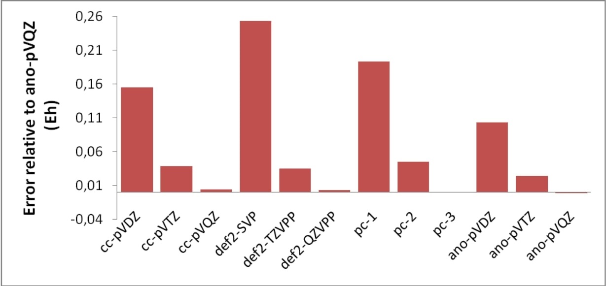
Fig. 6.4 Error in Eh for various basis sets for highly correlated calculations relative to the ano-pVQZ basis set.

Let us look at one more example in Table 6.4: the optimized structure of the N\(_2\) molecule as a function of basis set using the MP2 method (these calculations are a bit older from the time when the ano-pVnZ basis sets did not yet exist. Today, the ano-pVnZ would be preferred) .

The highest quality basis set here is QZVP and it also gives the lowest total energy. However, this basis set contains up to g-functions and is very expensive. Not using g-functions and a set of f-functions (as in TZVPP) has a noticeable effect on the outcome of the calculations and leads to an overestimation of the bond distance of 0.2 pm — a small change but for benchmark calculations of this kind still significant. The error made by the TZVP basis set that lacks the second set of d-functions on the bond distance, binding energy and ionization potential is surprisingly small even though the deletion of the second d-set “costs” more than 20 mEh in the total energy as compared to TZV(2d,2p), and even more compared to the larger TZVPP.

A significant error on the order of 1 – 2 pm in the calculated distances is produced by smaller DZP type basis sets, which underlines once more that such basis sets are really too small for correlated molecular calculations — the ANO-DZP basis sets are too strongly biased towards the atom, while the “usual” molecule targeted DZP basis sets like SVP have the d-set designed to cover polarization but not correlation (the correlating d-functions are steeper than the polarizing ones). The performance of the very economical SVP basis set should be considered as very good, and (a bit surprisingly) slightly better than cc-pVDZ despite that it gives a higher absolute energy.

Essentially the same picture is obtained by looking at the (uncorrected for ZPE) binding energy calculated at the MP2 level – the largest basis set, QZVP, gives the largest binding energy while the smaller basis sets underestimate it. The error of the DZP type basis sets is fairly large (\(\approx\) 2 eV) and therefore caution is advisable when using such bases.

Table 6.4 Comparison of various basis sets for correlated calculations.

Basis set	R\(_{\mathbf{eq} }\) (pm)	E(2N-N\(_{\mathbf{2} }\)) (eV)	IP(N/N\(^{\mathbf{+} }\)) (eV)	E(MP2) (Eh)
SVP	112.2	9.67	14.45	-109.1677
cc-pVDZ	112.9	9.35	14.35	-109.2672
TZVP	111.5	10.41	14.37	-109.3423
TZV(2d,2p)	111.4	10.61	14.49	-109.3683
TZVPP	111.1	10.94	14.56	-109.3973
QZVP	110.9	11.52	14.60	-109.4389

6.1.3.5. Automatic extrapolation to the basis set limit

Note

• This functionality is deprecated - it may still be usable but we will not actively maintain this part of code anymore. For basis set extrapolation please use the respective compound scripts (Table Protocols, known to the simple input line, with short explanation).

As eluded to in the previous section, one of the biggest problems with correlation calculations is the slow convergence to the basis set limit. One possibility to overcome this problem is the use of explicitly correlated methods. The other possibility is to use basis set extrapolation techniques. Since this involves some fairly repetitive work, some procedures were hardwired into the ORCA program. So far, only energies are supported. For extrapolation, a systematic series of basis sets is required. This is, for example, provided by the cc-pV\(n\)Z, aug-cc-pV\(n\)Z or the corresponding ANO basis sets. Here \(n\) is the “cardinal number” that is 2 for the double-zeta basis sets, 3 for triple-zeta, etc.

The convergence of the HF energy to the basis set limit is assumed to be given by:

(6.1)\[E_{\mathrm{SCF} }^{(X) } = E_{\mathrm{SCF} }^{(\infty) } + A \exp\left(-\alpha \sqrt{X}\right)\]

Here, \(E_{\mathrm{SCF} }^{(X) }\) is the SCF energy calculated with the basis set with cardinal number \(X\), \(E_{\mathrm{SCF} }^{(\infty) }\) is the basis set limit SCF energy and \(A\) and \(\alpha\) are constants. The approach taken in ORCA is to do a two-point extrapolation. This means that either \(A\) or \(\alpha\) have to be known. Here, we take \(A\) as to be determined and \(\alpha\) as a basis set specific constant.

The correlation energy is supposed to converge as:

(6.2)\[E_{\mathrm{corr} }^{(\infty) } = \frac{X^{\beta} E_{\mathrm{corr} }^{(X) } - Y^{\beta} E_{\mathrm{corr} }^{(Y) }}{X^{\beta} - Y^{\beta} } \]

The theoretical value for \(\beta\) is 3.0. However, it was found by Truhlar and confirmed by us, that for 2/3 extrapolations \(\beta = 2.4\) performs considerably better.

For a number of basis sets, we have determined the optimum values for \(\alpha\) and \(\beta\)[606]:

	\(\alpha_{\mathbf{23} }\)	\(\beta_{\mathbf{23} }\)	\(\alpha_{\mathbf{34} }\)	\(\beta_{\mathbf{34} }\)
cc-pVnZ	4.42	2.46	5.46	3.05
pc-n	7.02	2.01	9.78	4.09
def2	10.39	2.40	7.88	2.97
ano-pVnZ	5.41	2.43	4.48	2.97
saug-ano-pVnZ	5.48	2.21	4.18	2.83
aug-ano-pVnZ	5.12	2.41

Since the \(\beta\) values for 2/3 are close to 2.4, we always take this value. Likewise, all 3/4 and higher extrapolations are done with \(\beta=3\). However, the optimized values for \(\alpha\) are taken throughout.

Using the keyword ! Extrapolate(X/Y,basis), where X and Y are the corresponding successive cardinal numbers and basis is the type of basis set requested (= cc, aug-cc, cc-core, ano, saug-ano, aug-ano, def2) ORCA will calculate the SCF and optionally the MP2 or MDCI energies with two basis sets and separately extrapolate.

The keyword works also in the following way: ! Extrapolate(n,basis) where n is the is the number of energies to be used. In this way the program will start from a double-zeta basis and perform calculations with n cardinal numbers and then extrapolate the different pairs of basis sets. Thus for example the keyword ! Extrapolate(3,CC) will perform calculations with cc-pVDZ, cc-pVTZ and cc-pVQZ basis sets and then estimate the extrapolation results of both cc-pVDZ/cc-pVTZ and cc-pVTZ/cc-pVQZ combinations.

Let us take the example of the H2O molecule at the B3LYP/TZVP optimized geometry. The reference values have been determined from a HF calculation with the decontracted aug-cc-pV6Z basis set and the correlation energy was obtained from the cc-pV5Z/cc-pV6Z extrapolation. This gives:

E(SCF,CBS)           = -76.066958 Eh
EC(CCSD(T),CBS)      =  -0.30866 Eh
Etot(CCSD(T),CBS)    = -76.37561 Eh

Now we can see what extrapolation can bring in:

!CCSD(T) Extrapolate(2/3) TightSCF Conv Bohrs
* int 0 1
O 0 0 0  0 0 0
H 1 0 0  1.81975 0 0
H 1 2 0  1.81975 105.237 0
*

NOTE:

• The RI-JK and RIJCOSX approximations work well together with this option and RI-MP2 is also possible. Auxiliary basis sets are automatically chosen and can not be changed.

• All other basis set choices, externally defined bases etc. will be ignored — the automatic procedure only works with the default basis sets!

• The basis sets with the “core” postfix contain core correlation functions. By default it is assumed that this means that the core electrons are also to be correlated and the frozen core approximation is turned off. However, this can be overridden in the method block by choosing, e.g. %method frozencore fc_electrons end!

• So far, the extrapolation is only implemented for single points and not for gradients. Hence, geometry optimizations cannot be done in this way.

• The extrapolation method should only be used with very tight SCF convergence criteria. For open shell methods, additional caution is advised.

This gives:

Alpha(2/3)     :  4.420 (SCF Extrapolation)
Beta(2/3)      :  2.460 (correlation extrapolation)

SCF energy with basis cc-pVDZ:                          -76.026430944
SCF energy with basis cc-pVTZ:                          -76.056728252
Extrapolated CBS SCF energy (2/3) :                     -76.066581429 (-0.009853177) 

MDCI energy with basis cc-pVDZ:                          -0.214591061
MDCI energy with basis cc-pVTZ:                          -0.275383015
Extrapolated CBS correlation energy (2/3) :              -0.310905962 (-0.035522947)

Estimated CBS total energy (2/3) :                      -76.377487391

Thus, the error in the total energy is indeed strongly reduced. Let us look at the more rigorous 3/4 extrapolation:

Alpha(3/4)     :  5.460 (SCF Extrapolation)
Beta(3/4)      :  3.050 (correlation extrapolation)

SCF energy with basis cc-pVTZ:                          -76.056728252
SCF energy with basis cc-pVQZ:                          -76.064381269
Extrapolated CBS SCF energy (3/4) :                     -76.066687152 (-0.002305884) 

MDCI energy with basis cc-pVTZ:                          -0.275383016
MDCI energy with basis cc-pVQZ:                          -0.295324345
Extrapolated CBS correlation energy (3/4) :              -0.309520368 (-0.014196023)

Estimated CBS total energy (3/4) :                      -76.376207520

In our experience, the ANO basis sets extrapolate similarly to the cc-basis sets. Hence, repeating the entire calculation with Extrapolate(3,ANO) gives:

Estimated CBS total energy (2/3) :                      -76.377652792
Estimated CBS total energy (3/4) :                      -76.376983433

Which is within 1 mEh of the estimated CCSD(T) basis set limit energy in the case of the 3/4 extrapolation and within 2 mEh for the 2/3 extrapolation.

For larger molecules, the bottleneck of the calculation will be the CCSD(T) calculation with the larger basis set. In order to avoid this expensive (or prohibitive) calculation, it is possible to estimate the CCSD(T) energy at the basis set limit as:

(6.3)\[E_{\mathrm{corr} }^{(\mathrm{CCSD(T) };Y) } \approx E_{\mathrm{corr} }^{(\mathrm{CCSD(T) };X) } + E_{\mathrm{corr} }^{(\mathrm{MP2};\infty) } - E_{\mathrm{corr} }^{(\mathrm{MP2};X) } \]

This assumes that the basis set dependence of MP2 and CCSD(T) is similar. One can then extrapolate as before. Alternatively, the standard way — as extensively exercised by Hobza and co-workers — is to simply use:

(6.4)\[E_{\mathrm{total} }^{(\mathrm{CCSD(T) };\mathrm{CBS}) } \approx E_{\mathrm{SCF} }^{(Y) } + E_{\mathrm{corr} }^{(\mathrm{CCSD(T) };X) } + E_{\mathrm{corr} }^{(\mathrm{MP2};\infty) } - E_{\mathrm{corr} }^{(\mathrm{MP2};X) } \]

The appropriate keyword is:

! ExtrapolateEP2(2/3,ANO,MP2) TightSCF Conv Bohrs
* int 0 1
O 0 0 0  0 0 0
H 1 0 0  1.81975 0 0
H 1 2 0  1.81975 105.237 0
*

This creates the following output:

Alpha     :  5.410 (SCF Extrapolation)
Beta      :  2.430 (correlation extrapolation)

SCF energy with basis ano-pVDZ:                         -76.059178452
SCF energy with basis ano-pVTZ:                         -76.064774379
Extrapolated CBS SCF energy :                           -76.065995735 (-0.001221356) 

MP2 energy with basis ano-pVDZ:                          -0.219202871
MP2 energy with basis ano-pVTZ:                          -0.267058634
Extrapolated CBS correlation energy :                    -0.295568604 (-0.028509970)

CCSD(T) correlation energy with basis ano-pVDZ:          -0.229478341
CCSD(T) - MP2 energy with basis ano-pVDZ:                -0.010275470

Estimated CBS total energy :                            -76.371839809

The estimated correlation energy is not really bad — within 3 mEh from the basis set limit.

Using the ExtrapolateEP2(n/m,bas,[method, method-details]) keyword one can use a generalization of the above method where instead of MP2 any available correlation method can be used as described in Ref. [519]. method is optional and can be either MP2 or DLPNO-CCSD(T), the latter being the default. In case the method is DLPNO-CCSD(T) in the method-details option one can ask for LoosePNO, NormalPNO or TightPNO.

(6.5)\[E_{\mathrm{corr} }^{(\mathrm{CCSD(T) };CBS) } \approx E_{\mathrm{corr} }^{(\mathrm{CCSD(T) };X) } + E_{\mathrm{corr} }^{(\mathrm{M};CBS) }(X,X+1) - E_{\mathrm{corr} }^{(\mathrm{M};X) } \]

Here M represents any correlation method one would like to use. For the previous water molecule the input of a calculation that uses DLPNO-CCSD(T) (which is the default now) instead of MP2 would look like:

! ExtrapolateEP2(2/3,cc,DLPNO-CCSD(T)) TightSCF Conv Bohrs
* int 0 1
O 0 0 0  0 0 0
H 1 0 0  1.81975 0 0
H 1 2 0  1.81975 105.237 0
*

and it would produce the following output:

Alpha     :  4.420 (SCF Extrapolation)
Beta      :  2.460 (correlation extrapolation)

SCF energy with basis cc-pVDZ:                          -76.026430944
SCF energy with basis cc-pVTZ:                          -76.056728252
Extrapolated CBS SCF energy :                           -76.066581429 (-0.009853177) 

MDCI energy with basis cc-pVDZ:                          -0.214429497
MDCI energy with basis cc-pVTZ:                          -0.275299699
Extrapolated CBS correlation energy :                    -0.310868368 (-0.035568670)

CCSD(T) correlation energy with basis cc-pVDZ:           -0.214548320
CCSD(T) - MDCI energy with basis cc-pVDZ:                -0.000118824

Estimated CBS total energy :                            -76.377568621

which is less than 2 mEh from the basis set limit. Finally it was shown [519] that instead of extrapolating the cheap method, M, using cardinal numbers \(X\) and \(X+1\) it is better to use cardinal numbers \(X+1\) and \(X+2\).

(6.6)\[E_{\mathrm{corr} }^{(\mathrm{CCSD(T) };CBS) } \approx E_{\mathrm{corr} }^{(\mathrm{CCSD(T) };X) } + E_{\mathrm{corr} }^{(\mathrm{M};CBS) }(X+1,X+2) - E_{\mathrm{corr} }^{(\mathrm{M};X) } \]

This can be done using the ExtrapolateEP3(bas,[method,method-details]) keyword:

! ExtrapolateEP3(CC) TightSCF Conv Bohrs

and the corresponding output would be:

Alpha     :  5.460 (SCF Extrapolation)
Beta      :  3.050 (correlation extrapolation)

SCF energy with basis cc-pVDZ:                          -76.026430944
SCF energy with basis cc-pVTZ:                          -76.056728252
SCF energy with basis cc-pVQZ:                          -76.064381269
Extrapolated CBS SCF energy :                           -76.066687152 (-0.002305884) 

MDCI energy with basis cc-pVDZ:                          -0.214429497
MDCI energy with basis cc-pVTZ:                          -0.275299699
MDCI energy with basis cc-pVQZ:                          -0.295229871
Extrapolated CBS correlation energy :                    -0.309417951 (-0.014188080)

CCSD(T) correlation energy with basis cc-pVDZ:           -0.214548319
CCSD(T) - MDCI energy with basis cc-pVDZ:                -0.000118822

Estimated CBS total energy :                            -76.376223926

For the ExtrapolateEP2, and ExtrapolateEP3 keywords the default cheap method is the DLPNO-CCSD(T) with the NormalPNO thresholds. There also available options with MP2, and DLPNO-CCSD(T) with LoosePNO and TightPNO settings.

6.1.3.6. Explicitly Correlated MP2 and CCSD(T) Calculations

A physically perhaps somewhat more satisfying alternative to basis set extrapolation is the theory of explicit correlation. In this method terms are added to the wavefunction Ansatz that contain the interelectronic coordinates explicitly (hence the name “explicit correlation”). Initially these terms were linear in the interelectronic distances (“R12-methods”). However, it has later been found that better results can be obtained by using other functions, such as an exponential, of the interelectronic distance (“F12-methods”). These methods are known to yield near basis set limit results for correlation energies in conjunction with much smaller orbital basis sets.

In applying these methods several points are important:

• Special orbital basis sets are at least advantageous. The development of such basis sets is still in its infancy. For a restricted range of elements the basis sets cc-pV\(n\)Z-F12 are available (where \(n=\) D, T, Q) and are recommended. Note, that other than their names suggest, these are a fair bit larger than regular double, triple or quadruple-zeta basis sets

• In addition to an orbital basis set, a near-complete auxiliary basis set must be specified. This is the so-called “CABS” basis. For the three basis sets mentioned above these are called cc-pV\(n\)Z-F12-CABS. If you have elements that are not covered you are on your own to supply a CABS basis set. CABS basis sets can be read into ORCA in a way analogous to RI auxiliary basis sets (replace “AUX” by “CABS” in the input). There are automatic tools for building a CABS basis from an arbitrary orbital basis, e.g. AutoCABS[780]

• if the RI approximation is used in conjunction with F12, a third basis set is required - this can be the regular auxiliary “/C” basis, but we recommend to step one level up in the auxiliary basis set (e.g. use a cc-pVTZ/C fitting basis in conjunction with cc-pVDZ-F12)

• It is perfectly feasible to use RIJCOSX or RI-JK at the same time. In this case, you should provide a fourth basis set for the Coulomb fitting

• RHF and UHF are available, ROHF not. (Although, one can do a ROHF like calculation by using QROs)

• Gradients are not available

Doing explicitly correlated MP2 calculations is straightforward. For example look at the following calculation on the water molecule at a given geometry:

#
! F12-MP2 cc-pVDZ-F12 cc-pVDZ-F12-CABS  VeryTightSCF PModel 

* xyz 0 1
    O    0.000000000000     0.000000000000     0.369372944000 
    H    0.783975899000     0.000000000000    -0.184686472000 
    H   -0.783975899000     0.000000000000    -0.184686472000 
*

and similarly in conjunction with the RI approximation:

#
! F12-RI-MP2 cc-pVDZ-F12 cc-pVDZ-F12-CABS cc-pVTZ/C VeryTightSCF PModel 

* xyz 0 1
    O    0.000000000000     0.000000000000     0.369372944000 
    H    0.783975899000     0.000000000000    -0.184686472000 
    H   -0.783975899000     0.000000000000    -0.184686472000 
*

The output is relatively easy to interpret:

-----------------
RI-MP2-F12 ENERGY
-----------------

EMP2 correlation Energy            :      -0.241038994909
F12 correction                     :      -0.054735459470
                                        -----------------
MP2 basis set limit estimate       :      -0.295774454379

Hartree-Fock energy                :     -76.057963800414
(2)_S CABS correction to EHF       :      -0.003475342535
                                        -----------------
HF basis set limit estimate        :     -76.061439142949

MP2 total energy before F12        :     -76.299002795323
Total F12 correction               :      -0.058210802005
                                        -----------------
Final basis set limit MP2 estimate :     -76.357213597328

It consists of several parts. The first is the regular (RI-)MP2 correlation energy in the orbitals basis followed by the additive MP2 correction which are combined to provide an MP2 correlation energy basis set limit estimate. The second part consists of an estimate in the error in the underlying SCF energy. This is the “(2)_S CABS” correction. The combination of the SCF energy with this correction yields an estimate of the SCF basis set limit. The correction will typically undershoot somewhat, but the error is very smooth. Finally, the corrected correlation energy and the corrected SCF energy are added to yield the F12 total energy estimate at the basis set limit.

Let’s look at some results and compare to extrapolation:

#
# Correlation energies of the water molecule: extrapolation versus F12
#
# cc-pVDZ MP2: -0.201380894
#      T     : -0.261263141
#      Q     : -0.282661311
#     T/Q    : -0.298276192
#     Q/5    : -0.300598282
#  F12-DZ    : -0.295775804
#  RI-F12-DZ : -0.295933560 (cc-pVDZ/C)
#              -0.295774489 (cc-pVTZ/C)
#  F12-TZ    : -0.299164006
#  RI-F12-TZ : -0.299163478 (cc-pVQZ/C)
#  F12-QZ    : -0.300130086

It is obvious that extrapolated and F12 correlation energies converge to the same number (in this case around 300 mEh). The best extrapolated result is still below the F12 result (this would primarily be meaningful in a variational calculation). However, first of all this was an expensive extrapolation and second, the small residual F12 error is very smooth and cancels in energy differences. In any case, already the F12-double-zeta (where “double zeta” is to be interpreted rather loosely) brings one into within 5 mEh of the basis set limit correlation energy and the F12-triple-zeta calculation to within 1 mEh, which is impressive.

The additional effort for the F12 calculation is rather high, since five types of additional two-electron integrals need to be calculated. Both integrals in CABS space and in the original orbital (OBS) space must be calculated and mixed Fock matrices are also required. Hence, one may wonder, whether a double-zeta F12 calculation actually saves any time over, say, a quadruple-zeta regular calculation. The actual answer to this question is: “NO”. Given all possibilities of obtained approximate MP2 and SCF energies, we have investigated the question of how to obtain MP2 basis set limit energies most efficiently in some detail. The results show that in terms of timings, basis set extrapolation in combination with RI-JK is the method of choice for MP2.[521] However, energy differences are more reliable with F12-MP2. In combination with RI-JK or RIJCOSX F12-MP2 becomes also competitive in terms of computational efficiency.

This situation is different in the case of coupled-cluster methods, where F12 methods outperform extrapolation and are the method of choice.

For coupled-cluster theory, everything works in a very similar fashion:

# the keywords
! F12-CCSD(T)
# and
! CCSD(T)-F12
# are equivalent

A special feature of ORCA that can save large amounts of time, is to use the RI approximation only for the F12-part. The keyword here is:

! F12/RI-CCSD(T)
# or
! CCSD(T)-F12/RI

Everything else works as described for F12-MP2.

6.1.3.7. Frozen Core Options

In coupled-cluster calculations the Frozen Core (FC) approximation is applied by default. This implies that the core electrons are not included in the correlation treatment, since the inclusion of dynamic correlation in the core electrons usually affects relative energies insignificantly.

The frozen core option can be switched on or off with ! FrozenCore or ! NoFrozenCore in the simple input. More information and further options are given in section Frozen Core Options and in section Including (semi)core orbitals in the correlation treatment.

6.1.3.8. Local Coupled Pair and Coupled-Cluster Calculations

ORCA features a special set of local correlation methods. The prevalent local coupled-cluster approaches date back to ideas of Pulay and have been extensively developed by Werner, Schütz and co-workers. They use the concept of correlation domains in order to achieve linear scaling with respect to CPU, disk and main memory. While the central concept of electron pairs is very similar in both approaches, the local correlation methods in ORCA follow a completely different and original philosophy.

In ORCA rather than trying to use sparsity, we exploit data compression. To this end two concepts are used: (a) localization of internal orbitals, which reduces the number of electron pairs to be correlated since the pair correlation energies are known to fall off sharply with distance; (b) use of a truncated pair specific natural orbital basis to span the significant part of the virtual space for each electron pair. This guarantees the fastest convergence of the pair wavefunction and a nearly optimal convergence of the pair correlation energy while not introducing any real space cut-offs or geometrically defined domains. These PNOs have been used previously by the pioneers of correlation theory. However, as discussed in the original papers, the way in which they have been implemented into ORCA is very different. For a full description of technical details and numerical tests see:

• F. Neese, A. Hansen, D. G. Liakos: Efficient and accurate local approximations to the coupled-cluster singles and doubles method using a truncated pair natural orbital basis.[616]

• F. Neese, A. Hansen, F. Wennmohs, S. Grimme: Accurate Theoretical Chemistry with Coupled Electron Pair Models.[617]

• F. Neese, F. Wennmohs, A. Hansen: Efficient and accurate local approximations to coupled electron pair approaches. An attempt to revive the pair-natural orbital method.[622]

• D. G. Liakos, A. Hansen, F. Neese: Weak molecular interactions studied with parallel implementations of the local pair natural orbital coupled pair and coupled-cluster methods.[520]

• A. Hansen, D. G. Liakos, F. Neese: Efficient and accurate local single reference correlation methods for high-spin open-shell molecules using pair natural orbitals.[361]

• C. Riplinger, F. Neese: An efficient and near linear scaling pair natural orbital based local coupled-cluster method.[720]

• C. Riplinger, B. Sandhoefer, A. Hansen, F. Neese: Natural triple excitations in local coupled-cluster calculations with pair natural orbitals.[722]

• C. Riplinger, P. Pinski, U. Becker, E. F. Valeev, F. Neese: Sparse maps - A systematic infrastructure for reduced-scaling electronic structure methods. II. Linear scaling domain based pair natural orbital coupled cluster theory.[721]

• D. Datta, S. Kossmann, F. Neese: Analytic energy derivatives for the calculation of the first-order molecular properties using the domain-based local pair-natural orbital coupled-cluster theory[191]

• M. Saitow, U. Becker, C. Riplinger, E. F. Valeev, F. Neese: A new linear scaling, efficient and accurate, open-shell domain based pair natural orbital coupled cluster singles and doubles theory.[739]

In 2013, the so-called DLPNO-CCSD method (“domain based local pair natural orbital”) was introduced.[720] This method is near linear scaling with system size and allows for giant calculations to be performed. In 2016, significant changes to the algorithm were implemented leading to linear scaling with system size concerning computing time, hard disk and memory consumption.[721] The principal idea behind DLPNO is the following: it became clear early on that the PNO space for a given electron pair (ij) is local and located in the same region of space as the electron pair (ij). In LPNO-CCSD this locality was partially used in the local fitting to the PNOs (controlled by the parameter TCutMKN). However, the PNOs were expanded in canonical virtual orbitals which led to some higher order scaling steps. In DLPNO, the PNOs are expanded in the set of projected atomic orbitals:

\[\left|{ \tilde \mu } \right\rangle = \left( 1 - \sum\nolimits_i \left| i \right\rangle\left\langle i \right| \right)\left| \mu \right\rangle\]

where \(\left| \mu \right\rangle\) is an atomic orbital and \({\left| i \right\rangle}\) refers to an occupied molecular orbital. Such projected orbitals are an overcomplete representation of the virtual space. The projected orbital \(\left|{ \tilde \mu } \right\rangle\) is located in the same region of space as \(\left| \mu \right\rangle\) and hence can be assigned to atomic centers. This has first been invented and used by Pulay and Saebo [704] in their pioneering work on local correlation methods and widely exploited by Werner, Schütz and co-workers in their local correlation approaches. [754, 755] DLPNO-CCSD goes one step further in expanding the PNOs \(\left|{ \tilde a_{ij}^{} } \right\rangle\) of a given pair \((ij)\) as:

\[\left|{ \tilde a_{ij}^{} } \right\rangle = \sum\limits_{\tilde \mu \in \{ ij\} } { d_{\tilde \mu \tilde a}^{ij}\left|{ \tilde \mu } \right\rangle}\]

where \({\tilde \mu \in \{ ij\} }\) is the domain of atoms (range of \({\tilde \mu }\)) that is associated with the electron pair ij. The advantage of the PNO method is, that these domains can be chosen to be large (>15-20 atoms) without compromising the efficiency of the method.

The comparison between LPNO-CCSD and DLPNO-CCSD is shown in Fig. 6.5. It is obvious that DLPNO-CCSD is (almost) never slower than LPNO-CCSD. However, its true advantages do become most apparent for molecules with more than approximately 60 atoms. The triples correction, that was added with our second paper from 2013, shows a perfect linear scaling, as is shown in part (a) of Fig. 6.5. For large systems it adds about 10%–20% to the DLPNO-CCSD computation time, hence its addition is possible for all systems for which the latter can still be obtained. Since 2016, the entire DLPNO-CCSD(T) algorithm is linear scaling. The improvements of the linear-scaling algorithm, compared to DLPNO2013-CCSD(T), start to become significant at system sizes of about 300 atoms, as becomes evident in part (b) of Fig. 6.5.

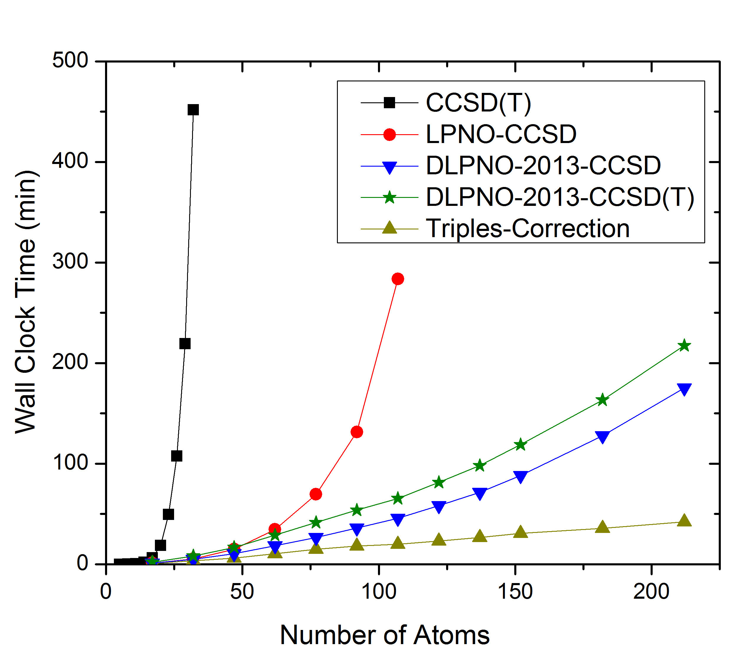(a) DLPNO2013 Scaling

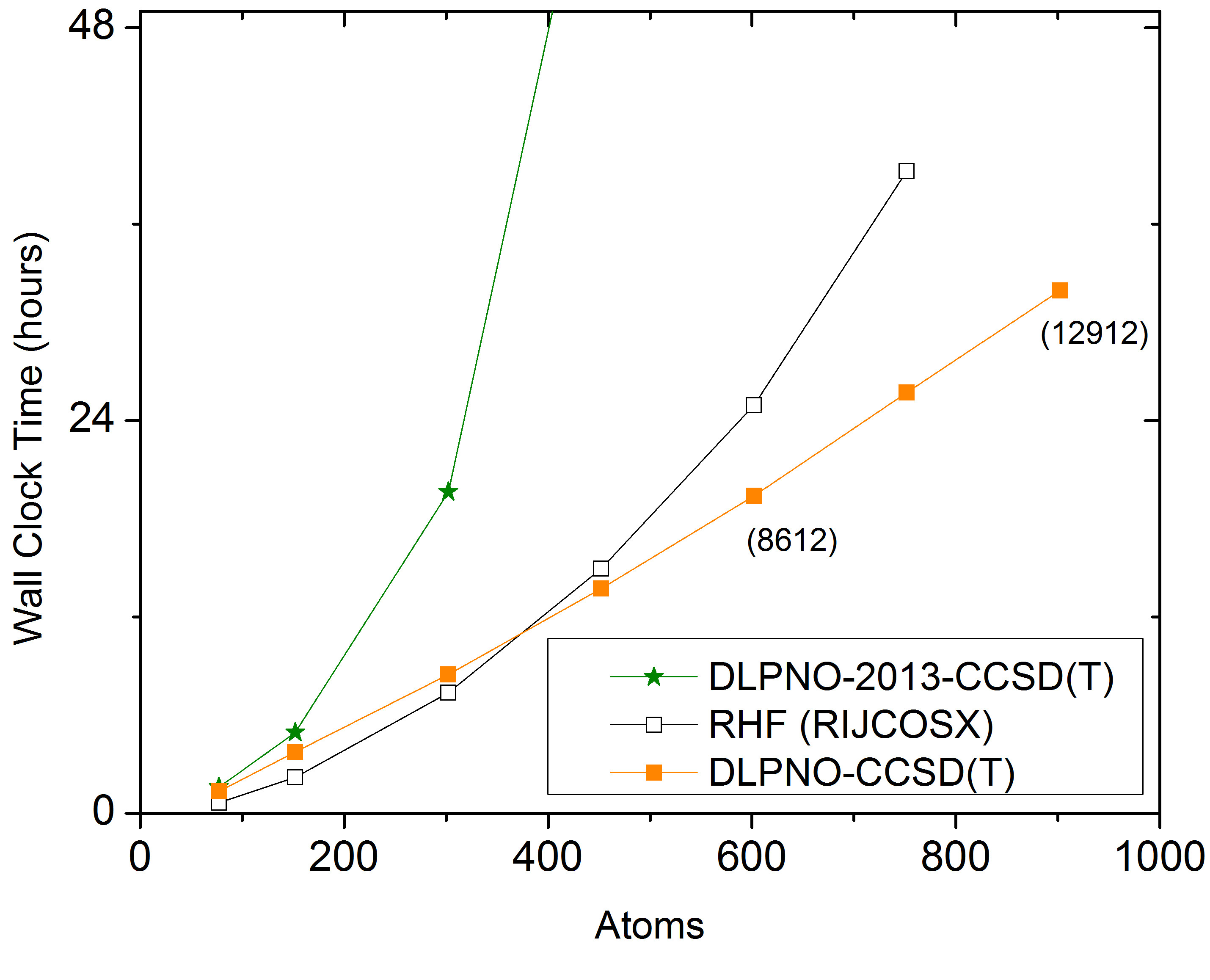(b) DLPNO Scaling

Fig. 6.5 a) Scaling behavior of the canonical CCSD, LPNO-CCSD and DLPNO2013-CCSD(T) methods. It is obvious that only DLPNO2013-CCSD and DLPNO2013-CCSD(T) can be applied to large molecules. The advantages of DLPNO2013-CCSD over LPNO-CCSD do not show before the system has reached a size of about 60 atoms. b) Scaling behavior of DLPNO2013-CCSD(T), DLPNO-CCSD(T) and RHF using RIJCOSX. It is obvious that only DLPNO-CCSD(T) can be applied to truly large molecules, is faster than the DLPNO2013 version, and even has a crossover with RHF at about 400 atoms.

Using the DLPNO-CCSD(T) approach it was possible for the first time (in 2013) to perform a CCSD(T) level calculation on an entire protein (Crambin with more than 650 atoms, Fig. 6.6). While the calculation using a double-zeta basis took about 4 weeks on one CPU with DLPNO2013-CCSD(T), it takes only about 4 days to complete with DLPNO-CCSD(T). With DLPNO-CCSD(T) even the triple-zeta basis calculation can be completed within reasonable time, taking 2 weeks on 4 CPUs.

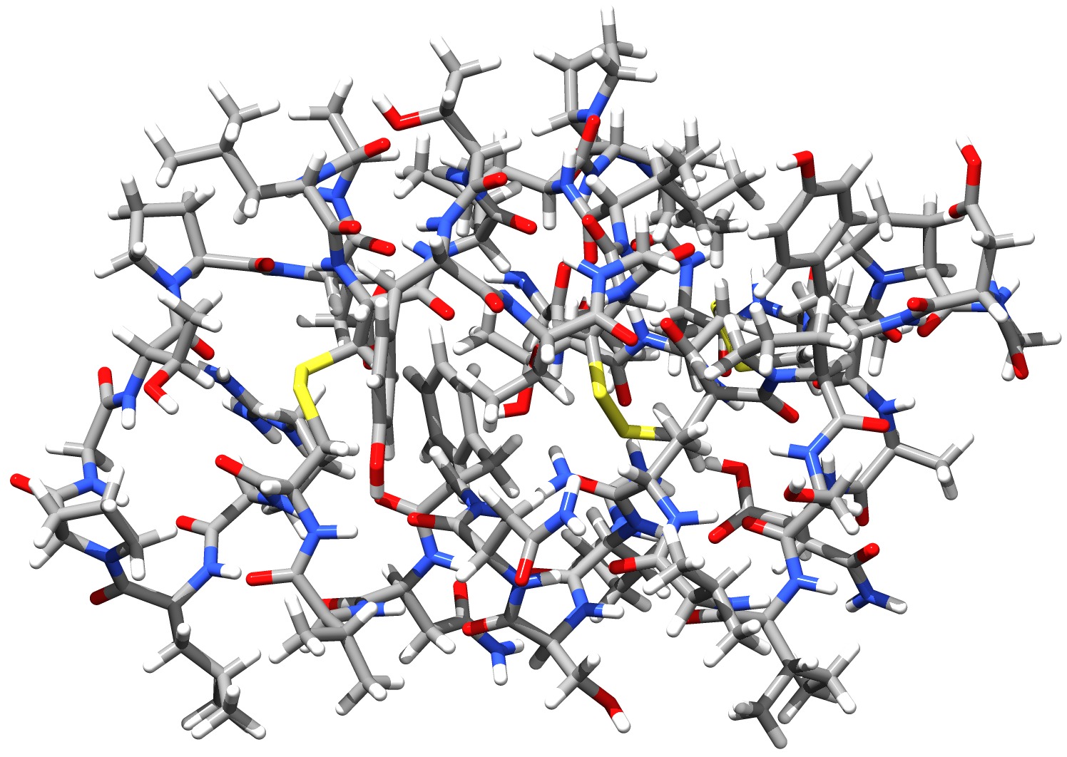
Fig. 6.6 Structure of the Crambin protein - the first protein to be treated with a CCSD(T) level ab initio method

The use of the LPNO (and DLPNO) methods is simple and requires little special attention from the user:

# Local Pair Natural Orbital Test
! cc-pVTZ cc-pVTZ/C LPNO-CCSD TightSCF
# or
! cc-pVTZ cc-pVTZ/C DLPNO-CCSD TightSCF
%maxcore 2000

# these are the default values - they need not to be touched!
%mdci  TCutPNO   3.33e-7   # cutoff for PNO occupation numbers. This
                             is the main truncation parameter
       TCutPairs 1e-4  # cut-off for estimated pair correlation energies.
                         This exploits the locality in the internal space
       TCutMKN   1e-3  # this is a technical parameter here that controls the domain
                         size for the local fit to the PNOs. It is conservative.
       end

* xyz 0 1
... (coordinates)
*

Using the well tested default settings, the LPNO-CEPA (LPNO-CPF, LPNO-VCEPA), LPNO-QCISD and LPNO-CCSD (LPNO-pCCSD) methods[6] can be run in strict analogy to canonical calculations and should approximate the canonical result very closely. In fact, one should not view the LPNO methods as new model chemistry - they are designed to reproduce the canonical results, including BSSE. This is different from the domain based local correlation methods that do constitute a new model chemistry with properties that are different from the original methods.

In some situations, it may be appropriate to adapt the accuracy of the calculation. Sensible defaults have been determined from extensive benchmark calculations and are accessible via LoosePNO, NormalPNO and TightPNO keywords in the simple input line.[522]

These keywords represent the recommended way to control the accuracy of DLPNO calculations as follows. Manual changing of thresholds beyond these specifying these keywords is usually discouraged.

# Tight settings for increased accuracy, e.g. when investigating
# weak interactions or conformational equilibria
! cc-pVTZ cc-pVTZ/C DLPNO-CCSD(T) TightPNO TightSCF

# OR: Default settings (no need to give NormalPNO explicitly)
# Useful for general thermochemistry
! cc-pVTZ cc-pVTZ/C DLPNO-CCSD(T) NormalPNO TightSCF

# OR: Loose settings for rapid estimates
! cc-pVTZ cc-pVTZ/C DLPNO-CCSD(T) LoosePNO TightSCF

%maxcore 2000

* xyz 0 1
... (coordinates)
*

Since ORCA 4.0, the linear-scaling DLPNO implementation described in reference [721] is the default DLPNO algorithm. However, for comparison, the first DLPNO implementation from references [720] and [722] can still be called by using the DLPNO2013 prefix instead of the DLPNO- prefix.

# DLPNO-CCSD(T) calculation using the 2013 implementation
! cc-pVTZ cc-pVTZ/C DLPNO2013-CCSD(T)

# DLPNO-CCSD(T) calculation using the linear-scaling implementation
! cc-pVTZ cc-pVTZ/C DLPNO-CCSD(T)

* xyz 0 1
... (coordinates)
*

Until ORCA 4.0, the “semi-canonical” approximation is used in the perturbative triples correction for DLPNO-CCSD. It was found that the “semi-canonical” approximation is a very good approximation for most systems. However, the “semi-canonical” approximation can introduce large errors in rare cases (particularly when the HOMO-LUMO gap is small), whereas the DLPNO-CCSD is still very accurate. To improve the accuracy of perturbative triples correction, since 4.1, an improved perturbative triples correction for DLPNO-CCSD is available, DLPNO-CCSD(T1)[341]. In DLPNO-CCSD(T1), the triples amplitudes are computed iteratively, which can reproduce more accurately the canonical (T) energies.

It is necessary to clarify the nomenclature used in ORCA input files. The keyword to invoke “semi-canonical” perturbative triples correction approximation is DLPNO-CCSD(T). While, the keyword of improved iterative approximation is DLPNO-CCSD(T1). However, in our recent paper[341], the “semi-canonical” perturbative triples correction approximation is named DLPNO-CCSD(T0), whereas the improved iterative one is called DLPNO-CCSD(T). Thus, the names used in our paper are different from those in ORCA input files. An example input file to perform improved iterative perturbative triples correction for DLPNO-CCSD is given below,

# DLPNO-CCSD(T1) calculation using the iterative triples correction
! cc-pVTZ cc-pVTZ/C DLPNO-CCSD(T1)

%mdci
      TNOSCALES    10.0 #TNO truncation scale for strong triples, TNOSCALES*TCutTNO.
                         Default setting is 10.0 
      TNOSCALEW   100.0 #TNO truncation scale for weak triples, TNOSCALEW*TCutTNO
                         Default setting is 100.0
      TriTolE      1e-4 #(T) energy convergence tolerance
                         Default setting is 1e-4
%end
* xyz 0 1
... (coordinates)
*

Since ORCA 4.2, the improved iterative perturbative triples correction for open-shell DLPNO-CCSD is available as well. The keyword of open-shell DLPNO-CCSD(T) is the same as that of the closed-shell case.

Since ORCA 4.0, the high-spin open-shell version of the DLPNO-CISD/QCISD/CCSD implementations have been made available on top of the same machinery as the 2016 version of the RHF-DLPNO-CCSD code. The present UHF-DLPNO-CCSD is designed to be an heir to the UHF-LPNO-CCSD and serves as a natural extension to the RHF-DLPNO-CCSD. A striking difference between UHF-LPNO and newly developed UHF-DLPNO methods is that the UHF-DLPNO approach gives identical results to that of the RHF variant when applied to closed-shell species while UHF-LPNO does not. Usage of this program is quite straightforward and shown below:

# (1) In case of ROHF reference
! ROHF DLPNO-CCSD def2-TZVPP def2-TZVPP/C TightSCF TightPNO

# (2) In case of UHF reference, the QROs are constructed first and used for
#     the open-shell DLPNO-CCSD computations
! UHF DLPNO-CCSD def2-TZVPP def2-TZVPP/C TightSCF TightPNO

# (3) In case that UKS is specified, the QROs are constructed first and used as
#     "unconverged" UHF orbitals for the open-shell DLPNO-CCSD computations.
#     This approach is useful when the converged UHF wavefunction is qualitatively
#     wrong but the UKS wavefunction is not
! UKS CAM-B3LYP DLPNO-CCSD def2-TZVPP def2-TZVPP/C TightSCF TightPNO

Note

DLPNO-CISD/QCISD/CCSD methods are dedicated to closed-shell and high-spin open-shell species, but not spin-polarized systems (e.g. open shell singlets or antiferromagnetically coupled transition metal clusters). Performing DLPNO-CISD/QCISD/CCSD calculations upon open shell singlet UHF/UKS wavefunctions will give results resembling the corresponding closed shell singlet calculations, because the DLPNO calculations will be done on the closed-shell determinant composed of the QRO orbitals. Similarly, calculations of spin-polarized systems other than open shell singlets may give qualitatively wrong results. For spin-polarized systems, the UHF-LPNO-CCSD or Mk-LPNO-CCSD methods are available, in addition to DLPNO-NEVPT2.

The same set of truncation parameters as closed-shell DLPNO-CCSD is used also in case of open-shell DLPNO. The open-shell DLPNO-CCSD produces more than 99.9 \(\%\) of the canonical CCSD correlation energy as in case of the closed-shell variant. This feature is certainly different from the UHF-LPNO methods because the open-shell DLPNO-CCSD is re-designed from scratch on the basis of a new PNO ansatz which makes use of the high-spin open-shell NEVPT framework. The computational timings of the UHF-DLPNO-CCSD and RIJCOSX-UHF for linear alkane chains in triplet state are shown in Fig. 6.7.

Fig. 6.7 Computational times of RIJCOSX-UHF and UHF-DLPNO-CCSD for the linear alkane chains (\(C_{n}H_{\text{2n + 2}}\)) in triplet state with def2-TZVPP basis and default frozen core settings. 4 CPU cores and 128 GB of memory were used on a single cluster node.

Although those systems are somewhat idealized for the DLPNO method to best perform, it is clear that the preceding RIJCOSX-UHF is the rate-determining step in the total computational time for large examples. In the open-shell DLPNO implementations, SOMOs are included not only in the occupied space but also in the PNO space in the preceding integral transformation step. This means the presence of more SOMOs may lead to more demanding PNO integral transformation and DLPNO-CCSD iterations. The illustrative examples include active site model of the [NiFe] Hydrogenase in triplet state and the oxygen evolving complex (OEC) in the high-spin state, which are shown in Figures 7 and 8, respectively. With def2-TZVPP basis set and NormalPNO settings, a single point calculation on [NiFe] Hydrogenase (Fig. 6.8) took approximately 45 hours on a single cluster node by using 4 CPU cores of Xeon E5-2670. A single point calculation on the OEC compound (Fig. 6.9) with the same computational settings finished in 44 hours even though the number of AOs in this system is even fewer than the Hydrogenase: the Hydrogenase active site model and OEC involve 4007 and 2606 AO basis functions, respectively. Special care should be taken if the system possesses more than ten SOMOs, since inclusion of more SOMOs may drastically increase the prefactor of the calculations. In addition, if the SOMOs are distributed over the entire molecular skeleton, each pair domain may not be truncated at all; in this case speedup attributed to the domain truncation will not be achieved at all.

Fig. 6.8 Ni-Fe active center in the [NiFe] Hydrogenase in its second-coordination sphere. The whole model system is composed of 180 atoms.

Fig. 6.9 A model compound for the OEC in the S\({}_2\) state of photosystem II which is composed of 238 atoms. In its high-spin state, the OEC possesses 13 SOMOs in total.

Calculation of the orbital-unrelaxed density has been implemented for closed-shell DLPNO-CCSD. This permits analytical computation of first-order properties, such as multipole moments or electric field gradients. In order to reproduce conventional unrelaxed CCSD properties to a high degree of accuracy, tighter thresholds may be needed than given by the default settings. Reading of the reference[191] is recommended. Calculation of the unrelaxed density is requested as usual:

%MDCI Density Unrelaxed End

There are a few things to be noticed about (D)LPNO methods:

• The LPNO methods obligatorily make use of the RI approximation. Hence, a correlation fit set must be provided.

• The DLPNO-CCSD(T) method is applicable to closed-shell or high-spin open-shell species. When performing DLPNO calculations on open-shell species, it is always better to have UCO option: If preceding SCF converges to broken-symmetry solutions, it is not guaranteed that the DLPNO-CCSD gives physically meaningful results.

• Besides the closed-shell version which uses a RHF or RKS reference determinant there is an open-shell version of the LPNO-CCSD for high-spin open-shell molecules (see original paper) using an UHF or UKS reference determinant built from quasi-restricted orbitals (QROs, see section Open-Shell Equations). Since the results of the current open-shell version are slightly less accurate than that of the closed-shell version it is mandatory to specify if you want to use the closed-shell or open-shell version for calculations of closed-shell systems, i.e. always put the “RHF” (“RKS”) or “UHF” (“UKS”) keyword in the simple keyword line. Open-shell systems can be of course only treated by the open-shell version. Do not mix results of the closed- and open-shell versions of LPNO methods (e.g. if you calculate reaction energies of a reaction in which both closed- and open-shell molecules take part, you should use the open-shell version throughout). This is because the open-shell LPNO results for the closed-shell species certainly differ from those of closed-shell implementations. This drawback of the open-shell LPNO methods has led to the development of a brand new open-shell DLPNO approach which converges to the RHF-DLPNO in the closed-shell limit. Importantly, one can mix the results of closed- and open-shell versions of DLPNO approaches.

• The open-shell version of the DLPNO approach uses a different strategy to the LPNO variant to define the open-shell PNOs. This ensures that, unlike the open-shell LPNO, the PNO space converges to the closed-shell counterpart in the closed-shell limit. Therefore, in the closed-shell limit, the open-shell DLPNO gives identical correlation energy to the RHF variant up to at least the third decimal place. The perturbative triples correction referred to as, (T), is also available for the open-shell species.

• When performing a calculation on the open-shell species with either of canonical/LPNO/DLPNO methods on top of the Slater determinant constructed from the QROs, special attention should be paid on the orbitals energies of those QROs. In some cases, the orbitals energy of the highest SOMO appear to be higher than that of the lowest VMO. Similarly to this, the orbital energy of the highest DOMO may appear to higher than that of the lowest SOMOs. In such cases, the CEPA/QCISD/CCSD iteration may show difficulty in convergence. In the worst case, it just diverges. Most likely, in such cases, one has to suspect the charge and multiplicity might be wrong. If they are correct, you may need much prettier starting orbitals and a bit of good luck! Apart from a careful choice of starting orbitals (in particular, DFT orbitals can be used in place of the default HF orbitals if the latter have qualitative deficiencies, including but not limited to severe spin contamination), changing the maximum DIIS expansion space size (MaxDIIS) and the level shift (LShift) in the %mdci block may alleviate the convergence problems to some extent.

• DLPNO-CCSD(T)-F12 and DLPNO-CCSD(T1)-F12 (iterative triples) are available for both closed- and open-shell cases. These methods employ a perturbative F12 correction on top of the DLPNO-CCSD(T) correlation energy calculation. The F12 part of the code uses the RI approximation in the same spirit as the canonical RI-F12 methods (refer to section Explicitly Correlated MP2 and CCSD(T) Calculations). Hence, they should be compared with methods using the RI approximation for both CC and F12 parts. The F12 correction takes only a fraction (usually 10-30%) of the total time (excluding SCF) required to calculate the DLPNO-CCSD(T)-F12 correlation energy. Thus, the F12 correction scales the same (linear or near-linear) as the parent DLPNO method. Furthermore, no new truncation parameters are introduced for the F12 procedure, preserving the black-box nature of the DLPNO method. The F12D approximation is highly recommended as it is computationally cheaper than the F12 approach which involves a double RI summation. Keywords: DLPNO-CCSD(T)-F12D, DLPNO-CCSD(T)-F12, DLPNO-CCSD(T1)-F12D, DLPNO-CCSD(T1)-F12, DLPNO-CCSD-F12D, DLPNO-CCSD-F12.

• Parallelization is done.

• There are three thresholds that can be user controlled that can all be adjusted in the %mdci block: (a) \(T_\text{CutPNO}\hspace{-0.25mm}\) controls the number of PNOs per electron pair. This is the most critical parameter and has a default value of \(3.33\times 10^{-7}\). (b) \(T_\text{CutPairs}\hspace{-0.25mm}\) controls a perturbative selection of significant pairs and has a default value of \(10^{-4}\). (c) \(T_\text{CutMKN}\hspace{-0.25mm}\) is a technical parameter and controls the size of the fit set for each electron pair. It has a default value of \(10^{-3}\). All of these default values are conservative. Hence, no adjustment of these parameters is necessary. All DLPNO-CCSD truncations are bound to these three truncation parameters and should almost not be touched (Hence they are also not documented :) ).

• The preferred way to adjust accuracy when needed is to use the “LoosePNO/NormalPNO/TightPNO” keywords. In addition, “TightPNO” triggers the full iterative (DLPNO-MP2) treatment in the MP2 guess, whereas the other options use a semicanonical MP2 calculation. Table 6.5 and Table 6.6 contain the thresholds used by the current (2016) and old (2013) implementations, respectively.

• LPNO-VCEPA/n (n=1,2,3) methods are only available in the open-shell version yet.

• LPNO variants of the parameterized coupled-cluster methods (pCCSD, see section Theory) are also available (e.g. LPNO-pCCSD/1a and LPNO-pC/2a).

• The LPNO methods reproduce the canonical energy differences to typically better than 1 kcal/mol. This accuracy exists over large parts of the potential energy surface. Tightening TCutPairs to 1e-5 gives more accurate results but also leads to significantly longer computation times.

• Potential energy surfaces are virtually but not perfectly smooth (like any method that involves cut-offs). Numerical gradient calculations have been attempted and reported to have been successful.

• The LPNO methods do work together with RIJCOSX, RI-JK and also with ANO basis sets and basis set extrapolation. They also work for conventional integral handling.

• The methods behave excellently with large basis sets. Thus, they stay efficient even when large basis sets are used that are necessary to obtain accurate results with wavefunction based ab initio methods. This is a prerequisite for efficient computational chemistry applications.

• For LPNO-CCSD, calculations with about 1000 basis functions are routine, calculations with about 1500 basis functions are possible and calculations with 2000-2500 basis functions are the limit on powerful computers. For DLPNO-CCSD much larger calculations are possible. There is virtually no crossover and DLPNO-CCSD is essentially always more efficient than LPNO-CCSD. Starting from about 50 atoms the differences become large. The largest DLPNO-CCSD calculation to date featured \(>\)1000 atoms and more than 20000 basis functions!

• Using large main memory is not mandatory but advantageous since it speeds up the initial integral transformation significantly (controlled by “MaxCore” in the %mdci block, see section Local correlation).

• The open-shell versions are about twice as expensive as the corresponding closed-shell versions.

• Analytic gradients are not available.

• An unrelaxed density implementation is available for closed-shell DLPNO-CCSD, permitting calculation of first-order properties.

Table 6.5 Accuracy settings for DLPNO coupled cluster (current version).

Setting	\(T_\text{CutPairs}\)	\(T_\text{CutDO}\)	\(T_\text{CutPNO}\)	\(T_\text{CutMKN}\)	MP2 pair treatment
LoosePNO	\(10^{-3}\)	\(2 \times 10^{-2}\)	\(1.00\times 10^{-6}\)	\(10^{-3}\)	semicanonical
NormalPNO	\(10^{-4}\)	\(1 \times 10^{-2}\)	\(3.33\times 10^{-7}\)	\(10^{-3}\)	semicanonical
TightPNO	\(10^{-5}\)	\(5 \times 10^{-3}\)	\(1.00\times 10^{-7}\)	\(10^{-3}\)	full iterative

Table 6.6 Accuracy settings for DLPNO coupled cluster (deprecated 2013 version).

Setting	\(T_\text{CutPairs}\)	\(T_\text{CutPNO}\)	\(T_\text{CutMKN}\)	MP2 pair treatment
LoosePNO	\(10^{-3}\)	\(1.00\times 10^{-6}\)	\(10^{-3}\)	semicanonical
NormalPNO	\(10^{-4}\)	\(3.33\times 10^{-7}\)	\(10^{-3}\)	semicanonical
TightPNO	\(10^{-5}\)	\(1.00\times 10^{-7}\)	\(10^{-4}\)	full iterative

As an example, see the following isomerization reaction that appears to be particularly difficult for DFT:

Isomerizes to:

The results of the calculations (closed-shell versions) with the def2-TZVP basis set (about 240 basis functions) are shown below:

Method	Energy Difference (kcal/mol)	Time (min)
CCSD(T)	-14.6	92.4
CCSD	-18.0	55.3
LPNO-CCSD	-18.6	20.0
CEPA/1	-12.4	42.2
LPNO-CEPA/1	-13.5	13.4

The calculations are typical in the sense that: (a) the LPNO methods provide answers that are within 1 kcal/mol of the canonical results, (b) CEPA approximates CCSD(T) more closely than CCSD. The speedups of a factor of 2 – 5 are moderate in this case. However, this is also a fairly small calculation. For larger systems, speedups of the LPNO methods compared to their canonical counterparts are on the order of a factor \(>\)100–1000.

6.1.3.9. Cluster in molecules (CIM)

Cluster in molecules (CIM) approach is a linear scaling local correlation method developed by Li and the coworkers in 2002.[514] It was further improved by Li, Piecuch, Kállay and other groups recently.[337, 340, 515, 516, 729] The CIM is inspired by the early local correlation method developed by Förner and coworkers.[250] The total correlation energy of a closed-shell molecule can be considered as a summation of correlation energies of each occupied LMOs.

(6.7)\[E_\text{corr}=\sum\limits_{i}^{occ}{E_{i} }=\sum\limits_{i}^{occ}{\frac{1}{4}\sum\limits_{j,ab} { \langle ij||ab\rangle } T_{ab}^{ij} } \]

For each occupied LMO, it only correlates with its nearby occupied LMOs and virtual MOs. To reproduce the correlation energy of each occupied LMO, only a subset of occupied and virtual LMOs are needed in the correlation calculation. Instead of doing the correlation calculation of the whole molecule, the correlation energies of all LMOs can be obtained within various subsystems.

The CIM approach implemented in ORCA is following an algorithm proposed by Guo and coworkers with a few improvements.[337, 340]

1. To avoid the real space cutoff, the differential overlap integral (DOI) is used instead of distance threshold. There is only one parameter ‘CIMTHRESH’ in CIM approach, controlling the construction of CIM subsystems. If the DOI between LMO i and LMO j is larger than CIMTHRESH, LMO j will be included into the MO domain of i. By including all nearby LMO of i, one can construct a subsystem for MO i. The default value of CIMTHRESH is 0.001. If accurate results are needed, a tighter CIMTHRESH must be used.

2. Since ORCA 4.1, the neglected correlations between LMO i and LMOs outside the MO domain of i are considered as well. These weak correlations are approximately evaluated by dipole moment integrals. With this correction, the CIM results of 3 dimensional proteins are significantly improved. About 99.8% of the correlation energies are recovered.

The CIM can invoke different single reference correlation methods for the subsystem calculations. In ORCA the CIM-RI-MP2, CIM-CCSD(T), CIM-DLPNO-MP2 and CIM-DLPNO-CCSD(T) methods are available. The CIM-RI-MP2 and CIM-DLPNO-CCSD(T) have been proved to be very efficient and accurate methods to compute correlation energies of very big molecules, containing a few thousand atoms.[340]
The usage of CIM in ORCA is simple. For CIM-RI-MP2,

#
# CIM-RI-MP2 calculation
#
! RI-MP2 cc-pVDZ cc-pVDZ/C CIM
%CIM
  CIMTHRESH 0.0005  # Default value is 0.001
end

* xyzfile 0 1 CIM.xyz

For CIM-DLPNO-CCSD(T),

#
# CIM-DLPNO-CCSD calculation
#
! DLPNO-CCSD(T) cc-pVDZ  cc-pVDZ/C CIM
* xyzfile 0 1 CIM.xyz

The parallel efficiency of CIM has been significantly improved.[340] Except for a few domain construction sub-steps, the CIM algorithm can achieve very high parallel efficiency. Since ORCA 4.1, the parallel version does not support Windows platform anymore due to the parallelization strategy. The generalization of CIM from closed-shell to open-shell (multi-reference) will also be implemented in the near future.

6.1.3.10. Arbitrary Order Coupled-Cluster Calculations

ORCA features an interface to Kallay’s powerful MRCC program. This program must be obtained separately. The interface is restricted to single point energies but can be used for rigid scan calculations or numerical frequencies.

The use of the interface is simple:

#
# Test the MRCC code of Mihael Kallay
#
! cc-pVDZ Conv SCFConv10 UseSym 

%mrcc method   "CCSDT"
      ETol     9
      end 

* xyz 0 1
F 0 0 0
H 0 0 0.95
*

The Method string can be any of:

# The excitation level specification can be anything
# like SD, SDT, SDTQ, SDTQP etc.
 %mrcc method   "CCSDT"
                "CCSD(T)"
                "CCSD[T]"
                "CCSD(T)_L"  (the lambda version)
                "CC3"
                "CCSDT-1a"
                "CCSDT-1b"
                "CISDT"

It is not a good idea, of course, to use this code for CCSD or CCSD(T) or CISD. Its real power lies in performing the higher order calculations. Open-shell calculations can presently not be done with the interface.

Note also that certain high-order configuration interaction or coupled cluster methods, such as CISDT, CISDTQ, CC3 and CCSDT etc., have now been implemented natively in ORCA in the AUTOCI module. For details please consult section CI methods using generated code.

6.1.4. Density Functional Theory

6.1.4.1. Standard Density Functional Calculations

Density functional calculations are as simple to run as HF calculations. In this case, the RI-J approximation will be the default for LDA, GGA or meta-GGA non-hybrid functionals, and the RIJCOSX for the hybrids. The RI-JK approximation might also offer large speedups for smaller systems.

For example, consider this B3LYP calculation on the cyclohexane molecule.

# Test a simple DFT calculation
! B3LYP SVP 
* xyz 0 1
C   -0.79263     0.55338    -1.58694
C    0.68078     0.13314    -1.72622
C    1.50034     0.61020    -0.52199
C    1.01517    -0.06749     0.77103
C   -0.49095    -0.38008     0.74228
C   -1.24341     0.64080    -0.11866
H    1.10490     0.53546    -2.67754
H    0.76075    -0.97866    -1.78666
H   -0.95741     1.54560    -2.07170
H   -1.42795    -0.17916    -2.14055
H   -2.34640     0.48232    -0.04725
H   -1.04144     1.66089     0.28731
H   -0.66608    -1.39636     0.31480
H   -0.89815    -0.39708     1.78184
H    1.25353     0.59796     1.63523
H    1.57519    -1.01856     0.93954
H    2.58691     0.40499    -0.67666
H    1.39420     1.71843    -0.44053
*

If you want an accurate single point energy then it is wise to choose “TightSCF” and select a basis set of at least valence triple-zeta plus polarization quality (e.g. def2-TZVP).

6.1.4.2. DFT Calculations with RI

DFT calculations that do not require the HF exchange to be calculated (non-hybrid DFT) can be very efficiently executed with the RI-J approximation. It leads to very large speedups at essentially no loss of accuracy. The use of the RI-J approximation may be illustrated for a medium sized organic molecule - Penicillin:

# RI-DFT calculation on the Penicillin molecule
! BP86 SVP TightSCF  

* xyz 0 1
N     3.17265     1.15815    -0.09175
C     2.66167     0.72032     1.18601
C     4.31931     0.59242    -0.73003
C     2.02252     1.86922    -0.54680
C     1.37143     1.52404     0.79659
S     2.72625    -1.05563     0.80065
C     4.01305    -0.91195    -0.52441
C     5.58297     1.09423    -0.06535
O     1.80801     2.36292    -1.62137
N     0.15715     0.73759     0.70095
C     5.25122    -1.72918    -0.12001
C     3.41769    -1.50152    -1.81857
O     6.60623     1.14077    -0.91855
O     5.72538     1.40990     1.08931
C    -1.08932     1.35001     0.75816
C    -2.30230     0.45820     0.54941
O    -1.19855     2.53493     0.96288
O    -3.48875     1.21403     0.57063
C    -4.66939     0.59150     0.27339
C    -4.84065    -0.79240     0.11956
C    -5.79523     1.39165     0.03916
C    -6.07568    -1.34753    -0.22401
C    -7.03670     0.85454    -0.30482
C    -7.18253    -0.52580    -0.43612
H     3.24354     1.09074     2.02120
H     4.33865     0.87909    -1.77554
H     1.26605     2.42501     1.39138
H     0.17381    -0.25857     0.47675
H     6.05024    -1.64196    -0.89101
H     5.67754    -1.39089     0.85176
H     5.01118    -2.81229    -0.01401
H     2.50304    -0.95210    -2.14173
H     4.15186    -1.44541    -2.65467
H     3.14138    -2.57427    -1.69700
H     7.29069     1.46408    -0.31004
H    -2.21049    -0.02915    -0.44909
H    -2.34192    -0.28647     1.37775
H    -4.00164    -1.48999     0.26950
H    -5.69703     2.48656     0.12872
H    -6.17811    -2.44045    -0.33185
H    -7.89945     1.51981    -0.47737
H    -8.15811    -0.96111    -0.71027
*

The job has 42 atoms and 430 contracted basis functions. Yet, it executes in just a few minutes elapsed time on any reasonable personal computer.

NOTES:

• The RI-J approximation requires an “auxiliary basis set” in addition to a normal orbital basis set. For the Karlsruhe basis sets there is the universal auxiliary basis set of Weigend that is called with the name def2/J (all-electron up to Kr). When scalar relativistic Hamiltonians are used (DKH or ZORA) along with all-electron basis sets, then a general-purpose auxiliary basis set is the SARC/J that covers most of the periodic table. Other choices are documented in sections Basis Sets and Choice of Basis Set.

• For “pure” functionals the use of RI-J with the def2/J auxiliary basis set is the default.

Since DFT is frequently applied to open-shell transition metals we also show one (more or less trivial) example of a Cu(II) complex treated with DFT.

! BP86 SV SlowConv  
%base "temp"
* xyz -2 2
  Cu  0     0     0
  Cl  2.25  0     0
  Cl -2.25  0     0
  Cl  0     2.25  0
  Cl  0    -2.25  0
*

$new_job

! B3LYP NoRI TZVP TightSCF MORead 
%moinp "temp.gbw"
%scf GuessMode CMatrix
     end
* xyz -2 2
  Cu  0     0     0
  Cl  2.25  0     0
  Cl -2.25  0     0
  Cl  0     2.25  0
  Cl  0    -2.25  0
*

Although it would not have been necessary for this example, it shows a possible strategy how to converge such calculations. First a less accurate but fast job is performed using the RI approximation, a GGA functional and a small basis set without polarization functions. Note that a larger damping factor has been used in order to guide the calculation (SlowConv). The second job takes the orbitals of the first as input and performs a more accurate hybrid DFT calculation. A subtle point in this calculation on a dianion in the gas phase is the command GuessMode CMatrix that causes the corresponding orbital transformation to be used in order to match the orbitals of the small and the large basis set calculation. This is always required when the orbital energies of the small basis set calculation are positive as will be the case for anions.

6.1.4.3. Hartree–Fock and Hybrid DFT Calculations with RIJCOSX

Frustrated by the large difference in execution times between pure and hybrid functionals, we have been motivated to study approximations to the Hartree-Fock exchange term. The method that we have finally come up with is called the “chain of spheres” COSX approximation and may be thought of as a variant of the pseudo-spectral philosophy. Essentially, in performing two electron integrals, the first integration is done numerically on a grid and the second (involving the Coulomb singularity) is done analytically. For algorithmic and theoretical details see Refs. [623] and [383]. Upon combining this treatment with the Split-RI-J method for the Coulomb term (thus, a Coulomb fitting basis is needed!), we have designed the RIJCOSX approximation that can be used to accelerate Hartree-Fock and hybrid DFT calculations. Note that this introduces another grid on top of the DFT integration grid which is usually significantly smaller.

OBS.: Since ORCA 5, RIJCOSX is the default option for hybrid DFT (can be turned off by using !NOCOSX). However, it is by default NOT turned on for HF.

In particular for large and accurate basis sets, the speedups obtained in this way are very large - we have observed up to a factor of sixty! The procedure is essentially linear scaling such that large and accurate calculations become possible with high efficiency. The RIJCOSX approximation is basically available throughout the program. The default errors are on the order of 0.05 \(\pm\) 0.1 kcal mol\(^{-1}\) or less in the total energies as well as in energy differences and can be made smaller with larger than the default grids or by running the final SCF cycle without this approximation. The impact on bond distances is a fraction of a pm, angles are better than a few tenth of a degree and soft dihedral angles are good to about 1 degree. To the limited extent to which it has been tested, vibrational frequencies are roughly good to 0.1 wavenumbers with the default settings.

The use of RIJCOSX is very simple:

! HF def2-TZVPP TightSCF RIJCOSX 
...

One thing to be mentioned in correlation calculations with RIJCOSX is that the requirements for the SCF and correlation fitting bases are quite different. We therefore support two different auxiliary basis sets in the same run:

! RI-MP2 def2-TZVPP def2/J def2-TZVPP/C TightSCF RIJCOSX
...

6.1.4.4. Hartree–Fock and Hybrid DFT Calculations with RI-JK

An alternative algorithm for accelerating the HF exchange in hybrid DFT or HF calculations is to use the RI approximation for both Coulomb and exchange. This is implemented in ORCA for SCF single point energies but not for gradients.

! RHF def2-TZVPP def2/JK RI-JK
...

The speedups for small molecules are better than for RIJCOSX, for medium sized molecules (e.g. \((\text{gly})_{4}\)) similar, and for larger molecules RI-JK is less efficient than RIJCOSX. The errors of RI-JK are usually below 1 mEh and the error is very smooth (smoother than for RIJCOSX). Hence, for small calculations with large basis sets, RI-JK is a good idea, for large calculations on large molecules RIJCOSX is better.

Note

• For RI-JK you will need a larger auxiliary basis set. For the Karlsruhe basis set, the universal def2/JK and def2/JKsmall basis sets are available. They are large and accurate.

• For UHF RI-JK is roughly twice as expensive as for RHF. This is not true for RIJCOSX.

• RI-JK is available for conventional and direct runs and also for ANO bases. There the conventional mode is recommended.

A comparison of the RIJCOSX and RI-JK methods (taken from Ref. [465]) for the \(\text{(gly)}_{2}\), \(\text{(gly)}_{4}\) and \(\text{(gly)}_{8}\) is shown below (wall clock times in second for performing the entire SCF):

		Def2-SVP	Def2-TZVP(-df)	Def2-TZVPP	Def2-QZVPP
\(\text{(gly)}_{2}\)	Default	105	319	2574	27856
	RI-JK	44	71	326	3072
	RIJCOSX	70	122	527	3659
\(\text{(gly)}_{4}\)	Default	609	1917	13965	161047
	RI-JK	333	678	2746	30398
	RIJCOSX	281	569	2414	15383
\(\text{(gly)}_{8}\)	Default	3317	12505	82774
	RI-JK	3431	5452	16586	117795
	RIJCOSX	1156	2219	8558	56505

It is obvious from the data that for small molecules the RI-JK approximation is the most efficient choice. For \(\text{(gly)}_{4}\) this is already no longer obvious. For up to the def2-TZVPP basis set, RI-JK and RIJCOSX are almost identical and for def2-QZVPP RIJCOSX is already a factor of two faster than RI-JK. For large molecules like \(\text{(gly)}_{8}\) with small basis sets RI-JK is not a big improvement but for large basis set it still beats the normal 4-index calculation. RIJCOSX on the other hand is consistently faster. It leads to speedups of around 10 for def2-TZVPP and up to 50-60 for def2-QZVPP. Here it outperforms RI-JK by, again, a factor of two.

6.1.4.5. DFT Calculations with Second Order Perturbative Correction (Double-Hybrid Functionals)

There is a family of functionals which came up in 2006 and were proposed by Grimme [320]. They consist of a semi-empirical mixture of DFT components and the MP2 correlation energy calculated with the DFT orbitals and their energies. Grimme referred to his functional as B2PLYP (B88 exchange, 2 parameters that were fitted and perturbative mixture of MP2 and LYP) – a version with improved performance (in particular for weak interactions) is mPW2PLYP [772] and is also implemented. From the extensive calibration work, the new functionals appear to give better energetics and a narrower error distribution than B3LYP. Thus, the additional cost of the calculation of the MP2 energy may be well invested (and is quite limited in conjunction with density fitting in the RI part). Martin has reported reparameterizations of B2PLYP (B2GP-PLYP, B2K-PLYP and B2T-PLYP) that are optimized for “general-purpose”, “kinetic” and “thermochemistry” applications.[436, 843] In 2011, Goerigk and Grimme published the PWPB95 functional with spin-opposite-scaling and relatively low amounts of Fock exchange, which make it promising for both main-group and transition-metal chemistry. [308]

Among the best performing density functionals[312] are Martin’s “DSD”-double-hybrids, which use different combinations of exchange and correlation potentials and spin-component-scaled MP2 mixing. Three of these double-hybrids (DSD-BLYP, DSD-PBEP86 and DSD-PBEB95)[467, 468, 469] are available via simple input keywords. Different sets of parameters for the DSD-double-hybrids are published, e.g. for the use with and without D3. The keywords DSD-BLYP, DSD-PBEP86 and DSD-PBEB95 request parameters consistent with the GMTKN55[312] benchmark set results. The keywords DSD-BLYP/2013 and DSD-PBEP86/2013 request the slightly different parameter sets used in the 2013 paper by Kozuch and Martin.[469] To avoid confusion, the different parameters are presented in Table 6.7.

Table 6.7 DSD-DFT parameters defined in ORCA

Keywords	ScalDFX	ScalHFX	ScalGGAC	PS	PT	D3S6	D3S8	D3A2
DSD-BLYP	0.25	0.75	0.53	0.46	0.60
DSD-BLYP D3BJ	0.31	0.69	0.54	0.46	0.37	0.50	0.213	6.0519
DSD-BLYP/2013 D3BJ	0.29	0.71	0.54	0.47	0.40	0.57	0	5.4
DSD-PBEP86	0.28	0.72	0.44	0.51	0.36
DSD-PBEP86 D3BJ	0.30	0.70	0.43	0.53	0.25	0.418	0	5.65
DSD-PBEP86/2013 D3BJ	0.31	0.69	0.44	0.52	0.22	0.48	0	5.6
DSD-PBEB95	0.30	0.70	0.52	0.48	0.22
DSD-PBEB95 D3BJ	0.34	0.66	0.55	0.46	0.09	0.61	0	6.2

Note that D3A1 is always 0 for these functionals.

Three different variants of MP2 can be used in conjunction with these functionals. Just specifying the functional name leads to the use of RI-MP2 by default. In this case, an appropriate auxiliary basis set for correlation fitting needs to be specified. It is very strongly recommended to use the RI variants instead of conventional MP2, as their performance is vastly better. Indeed, there is hardly ever any reason to use conventional MP2. To turn this option off just use !NORI in the simple input (which also turns off the RIJCOSX approximation) or %mp2 RI false end. More information can be found in the relevant sections regarding RI-MP2.

Finally, DLPNO-MP2 can be used as a component of double-hybrid density functionals. In that case, a “DLPNO-” prefix needs to be added to the functional name, for example DLPNO-B2GP-PLYP or DLPNO-DSD-PBEP86. Please refer to the relevant manual sections for more information on the DLPNO-MP2 method.

For each functional, parameters can be specified explicitly in the input file, e.g. for RI-DSD-PBEB95 with D3BJ:

! D3BJ
%method
  Method      DFT
  DoMP2       True
  Exchange    X_PBE
  Correlation C_B95
  LDAOpt      C_PWLDA # specific for B95
  ScalDFX     0.34
  ScalHFX     0.66
  ScalGGAC    0.55
  ScalLDAC    0.55 # must be equal to ScalGGAC
  ScalMP2C    1.00 # for all DSD-DFs
  D3S6        0.61
  D3S8        0
  D3A1        0    # for all DSD-DFs
  D3A2        6.2
end
%mp2
  DoSCS       True
  RI          True
  PS          0.46
  PT          0.09
end

In this version of ORCA, double-hybrid DFT is available for single points, geometry optimizations [619], dipole moments and other first order properties, magnetic second order properties (chemical shifts, g-tensors), as well as for numerical polarizabilities and frequencies.

There are also double-hybrid functionals, such as XYG3 and \(\omega\)B97M(2), which must be applied to orbitals converged with a different functional. This can be accomplished with a two-step calculation using MORead and MaxIter=1. Note that because the orbitals are not obtained self-consistently, only single point energies can be computed in this way, i.e. no density, gradient, or properties! For example, the \(\omega\)B97M(2) functional must be used with \(\omega\)B97M-V orbitals,[557] which can be done with the following input:

*xyz 0 1
  H 0.0 0.0 0.0
  F 0.0 0.0 0.9
*
%compound
  Variable EwB97MV, EwB97M2; # Output variables
  # Step 1: wB97M-V calculation to obtain the orbitals
  New_Step
    ! wB97M-V SCNL def2-TZVP
  Step_End
  # Step 2: single iteration with the wB97M(2) functional 
  #         + MP2 correlation to get the final energy
  ReadMOs(1);
  New_Step
    ! wB97M(2) SCNL NoFrozenCore def2-TZVP def2-TZVP/C
    %scf
      MaxIter    1
      IgnoreConv 1 # prevent the "not converged" error
    end
  Step_End
  Read EwB97MV = DFT_Total_En[1];     # wB97M-V energy
  Read EwB97M2 = MP2_Total_Energy[2]; # wB97M(2) energy
End

6.1.4.6. DFT Calculations with Atom-pairwise Dispersion Correction

It is well known that many DFT functionals do not include dispersion forces. It is possible to use a simple atom-pairwise correction to account for the major parts of this contribution to the energy [131, 321, 324, 326]. We have adopted the code and method developed by Stefan Grimme in this ORCA version. The method is parameterized for many established functionals (e.g. BLYP, BP86, PBE, TPSS, B3LYP, B2PLYP).[7] For the 2010 model the Becke-Johnson damping version (! D3BJ) is the default and will automatically be invoked by the simple keyword ! D3. The charge dependent atom-pairwise dispersion correction (keyword ! D4) is using the D4(EEQ)-ATM dispersion model[132], other D4 versions, using tight-binding partial charges, are currently only available with the standalone DFT-D4 program.

! BLYP D3 def2-QZVPP Opt

%paras R= 2.5,4.0,16
end

%geom Constraints
      { C 0 C }
      { C 1 C }
      end
end

* xyz 0 1
Ar    0.0000000    0.0000000    {R}
H     0.0000000    0.0000000    0.0000000
C     0.0000000    0.0000000   -1.0951073
H     0.5163499    0.8943443   -1.4604101
H     0.5163499   -0.8943443   -1.4604101
H    -1.0326998    0.0000000   -1.4604101
*

In this example, a BLYP calculation without dispersion correction will show a repulsive potential between the argon atom and the methane molecule. Using the D3 dispersion correction as shown above, the potential curve shows a minimum at about 3.1\(-\)3.2 Å. The atom-pairwise correction is quite successful and Grimme’s work suggests that this is more generally true. For many systems like stacked DNA base pairs, hydrogen bond complexes and other weak interactions the atom-pairwise dispersion correction will improve substantially the results of standard functionals at essentially no extra cost.

Note

• Dispersion corrections do not only affect non-covalent complexes, but also affect conformational energies (and conformer structures) which are heavily influenced by intramolecular dispersion. Therefore, for large and/or flexible molecules, including the dispersion correction is almost always recommended or even required (except for a handful of cases where it cannot, should not or need not be used, see below). For small systems, the dipersion correction may result in basically no improvement of the results, but is usually harmless anyway.

• DFT calculations with small basis sets (such as double zeta basis sets) often yield attractive potential energy surfaces even without the dispersion correction. However, this is due to basis set superposition error (BSSE), and the interaction energy brought about by the BSSE frequently does not match the true interaction energy due to dispersion (because they have completely different origins). Therefore, although a DFT double zeta calculation without the dispersion correction may appear to give qualitatively correct results, or occasionally even better results than a double zeta calculation with dispersion corrections (because in the latter case one typically overestimates the total attraction), it is still highly recommended to “get the right answer for the right reason” by reducing the BSSE and turning on the dispersion correction. The BSSE can be corrected by a variety of means, for example (1) by using a larger basis set; (2) by using the counterpoise correction (Counterpoise Correction); or (3) by using the geometrical counterpoise correction (section DFT and HF Calculations with the Geometrical Counterpoise Correction: gCP). Of these, (3) is available at almost no cost (including analytic gradient contributions), and is especially suitable for geometry optimization of large molecules. Otherwise (1) (or its combination with (2)) may be more appropriate due to its higher accuracy.

• Functionals that contain VV10-type non-local dispersion (in general, these are the functionals whose names end with “-V”) do not need (and cannot be used together with) dispersion corrections. The same holds for post-HF and multireference methods, like MP2, CCSD(T), CASSCF and NEVPT2. However, one can add a dispersion correction on top of HF.

• Certain functionals, especially the Minnesota family of functionals (e.g. M06-2X), describe medium-range dispersion but miss long-range dispersion. They give reasonable dispersion energies for small to medium systems but may slightly underestimate the dispersion energies for large systems. For them, dispersion corrections are only available in the zero-damping variant, and one should use the D3ZERO keyword instead of the D3 keyword. As the uncorrected functional already accounts for the bulk of the dispersion in this case, the dispersion correction is much less important than e.g. the case of B3LYP, and should in general be considered as beneficial but not mandatory.

• Some density functional developers reparameterize the functional itself while parameterizing the dispersion correction. A famous example is the \(\omega\)B97X family of functionals, to be detailed in the next section. For these functionals, the D3, D3BJ or D4 keywords should be hyphenated with the name of the functional itself, and some quantities that normally would not change when adding dispersion corrections (e.g. orbitals, excitation energies, dipole moments) may change slightly when adding or removing the dispersion correction. Likewise, for these functionals the structural changes that one observe upon adding or removing the dispersion correction cannot be completely attributed to the dispersion correction itself, but may contain contributions due to the change of the functional.

6.1.4.7. DFT Calculations with Range-Separated Hybrid Functionals

All range-separated functionals in ORCA use the error function based approach according to Hirao and coworkers.[410] This allows the definition of DFT functionals that dominate the short-range part by an adapted exchange functional of LDA, GGA or meta-GGA level and the long-range part by Hartree-Fock exchange.

CAM-B3LYP,[899] LC-BLYP[845], LC-PBE[410, 601] and members of the \(\omega\)B97-family of functionals have been implemented into ORCA, namely \(\omega\)B97, \(\omega\)B97X[151], \(\omega\)B97X-D3[525], \(\omega\)B97X-V[554], \(\omega\)B97M-V[556], \(\omega\)B97X-D3BJ and \(\omega\)B97M-D3BJ.[602] (For more information on \(\omega\)B97X-V[554] and \(\omega\)B97M-V[556] see section DFT Calculations with the Non-Local, Density Dependent Dispersion Correction (VV10): DFT-NL.) Some of them incorporate fixed amounts of Hartree-Fock exchange (EXX) and/or DFT exchange and they differ in the RS-parameter \(\mu\). In the case of \(\omega\)B97X-D3, the proper D3 correction (employing the zero-damping scheme) should be calculated automatically. The D3BJ correction is used automatically for \(\omega\)B97X-D3BJ and \(\omega\)B97M-D3BJ (as well as for the meta-GGA B97M-D3BJ). The same is true for the D4-based variants \(\omega\)B97M-D4 and \(\omega\)B97X-D4. The D3BJ and D4 variants have also been shown to perform well for geometry optimizations [603].

Several restrictions apply to these functionals at the moment. They have only been implemented and tested for use with the libint integral package and for RHF and UHF single-point, ground state nuclear gradient, ground state nuclear Hessian, TDDFT, and TDDFT nuclear gradient calculations. Only the standard integral handling (NORI), RIJONX, and RIJCOSX are supported. Do not use these functionals with any other options.

6.1.4.8. DFT Calculations with Range-Separated Double Hybrid Functionals

For the specifics of the range-separated double-hybrid functionals the user is referred to sections DFT Calculations with Second Order Perturbative Correction (Double-Hybrid Functionals), DFT Calculations with Range-Separated Hybrid Functionals and Doubles Correction. The first range-separated double hybrids available in ORCA were \(\omega\)B2PLYP and \(\omega\)B2GP-PLYP[146]. Both were optimized for the calculation of excitation energies, but they have recently also been tested for ground-state properties[601].

A large variety of range-separated double hybrids with and without spin-component/opposite scaling have become available in ORCA 5. Some have been developed with ground-state properties in mind, most for excitation energies. See Section Choice of Functional for more details and citations.

6.1.5. Quadratic Convergence

The standard SCF implementation in ORCA uses the DIIS algorithm[702, 703] for initial and an approximate second-order converger for final convergence[264, 607]. This approach converges quickly for most chemical systems. However, there are many interesting systems with a more complicated electronic structure for which the standard SCF protocol converges either slowly (“creeping”), converges to an excited state, or diverges. In those cases, a newly developed trust-region augmented Hessian (TRAH) SCF approach[64, 349, 381, 734] should be used. The TRAH-SCF method always converges to a local minimum and converges quadratically near the solution.

You can run TRAH from the beginning by adding

! TRAH

to the simple input line if you expect convergence difficulties. Open-shell molecules notoriously have SCF convergence issues, in particular, if they are composed of many open-shell atoms. In Fig. 6.10, the convergence of a TRAH-SCF calculation is shown for a high-spin Rh cluster for which the standard SCF diverges. The errors of the electronic gradient or residual vector converge almost steadily below the default TRAH accuracy of \(10^{-6}\).

Fig. 6.10 TRAH-SCF gradient norm of a PBE/def2-TZVP calculation for a \(\mathrm{Rh}_{12}^+\) cluster in high-spin configuration (\(\mathrm{M_s} = 36\)). The structure was taken from Ref. [362].

Alternatively, TRAH is launched automatically if standard SCF (DIIS/SOSCF) shows converge problems (default), an approach which is called AutoTRAH.

%scf
 AutoTRAH true
end

You can switch off the automatic start of TRAH by adding

! NOTRAH

to the simple input line or

%scf
 AutoTRAH false
end

Convergence problems are detected by comparing the norm of the electronic gradient at multiple iterations which is explained in more detail in Sec. Trust-Region Augmented Hessian (TRAH) SCF.

TRAH-SCF is currently implemented for restricted closed-shell (RHF and RKS) and unrestricted open-shell determinants (UHF and UKS) and can be accelerated with RIJ, RIJONX, RIJK, or RIJCOSX. Solvation effects can also be accounted for with the C-PCM and SMD models. Restricted open-shell calculations are not possible yet.

TRAH-SCF can also be applied to large molecules as it is parallelized and works with AO Fock matrices. However, for systems with large HOMO-LUMO gaps that converge well, the default SCF converger is usually faster because the screening in TRAH is less effective and more iterations are required.

For a more detailed documentation we refer to Sec. Trust-Region Augmented Hessian (TRAH) SCF.

Note

• TRAH is mathematically guaranteed to converge with a sufficient number of iterations, provided that there is no numerical noise (e.g. round-off error, truncation error) in the calculation. Therefore, if TRAH fails to converge, this means that either the default number of iterations is not large enough, or certain numerical thresholds are not tight enough. One can verify whether the former possibility is operative by checking whether the error still decreases steadily towards zero in the last SCF iterations. If yes, one can increase the number of iterations; otherwise it may be worthwhile to try increasing the integration grid, tighten the integral thresholds, etc.

• For some functionals (e.g. PWPB95), the native ORCA implementation supports only their XC energies and potentials, but not their XC kernels. In this case one should switch to the LibXC implementation instead, e.g. replace PWPB95 by LIBXC(PWPB95). Otherwise the calculation aborts upon entering the TRAH procedure.

6.1.6. Counterpoise Correction

In calculating weak molecular interactions the nasty subject of the basis set superposition error (BSSE) arises. It consists of the fact that if one describes a dimer, the basis functions on A help to lower the energy of fragment B and vice versa. Thus, one obtains an energy that is biased towards the dimer formation due to basis set effects. Since this is unwanted, the Boys and Bernardi procedure aims to correct for this deficiency by estimating what the energies of the monomers would be if they had been calculated with the dimer basis set. This will stabilize the monomers relative to the dimers. The effect can be a quite sizable fraction of the interaction energy and should therefore be taken into account. The original Boys and Bernardi formula for the interaction energy between fragments A and B is:

(6.8)\[ \Delta E = E^{AB}_{AB}(AB) - E^{A}_{A}(A) - E^{B}_{B}(B) - \left[E^{AB}_{A}(AB) - E^{AB}_{A}(A) + E^{AB}_{B}(AB) - E^{AB}_{B}(B)\right] \]

Here \(E_{X}^{Y} \left( Z \right)\) is the energy of fragment X calculated at the optimized geometry of fragment Y with the basis set of fragment Z. Thus, you need to do a total the following series of calculations:

1. optimize the geometry of the dimer and the monomers with some basis set Z. This gives you \(E_{AB}^{AB} \left({ AB} \right)\), \(E_{A}^{A} \left( A \right)\) and \(E_{B}^{B} \left( B \right)\)

2. delete fragment A (B) from the optimized structure of the dimer and re-run the single point calculation with basis set Z. This gives you \(E_{B}^{AB} \left( B \right)\) and \(E_{A}^{AB} \left( A \right)\).

3. Now, the final calculation consists of calculating the energies of A and B at the dimer geometry but with the dimer basis set. This gives you \(E_{A}^{AB} \left({ AB} \right)\) and \(E_{B}^{AB} \left({ AB} \right)\).

In order to achieve the last step efficiently, a special notation was put into ORCA which allows you to delete the electrons and nuclear charges that come with certain atoms but retain the assigned basis set. This trick consists of putting a “:” after the symbol of the atom. Here is an example of how to run such a calculation of the water dimer at the MP2 level (with frozen core):

#
# BSSE test
#

# --------------------------------------------
# First the monomer. It is a waste of course
# to run the monomer twice ...
# --------------------------------------------
! RHF MP2 TZVPP VeryTightSCF XYZFile PModel
%id "monomer"
* xyz 0 1
 O     7.405639     6.725069     7.710504
 H     7.029206     6.234628     8.442160
 H     8.247948     6.296600     7.554030
*

$new_job
! RHF MP2 TZVPP VeryTightSCF XYZFile PModel
%id "monomer"
* xyz 0 1
 O     7.405639     6.725069     7.710504
 H     7.029206     6.234628     8.442160
 H     8.247948     6.296600     7.554030
*

# --------------------------------------------
# now the dimer
# --------------------------------------------
$new_job
! RHF MP2 TZVPP VeryTightSCF XYZFile PModel
%id "dimer"
* xyz 0 1
O   7.439917   6.726792   7.762120
O   5.752050   6.489306   5.407671
H   7.025510   6.226170   8.467436
H   8.274883   6.280259   7.609894
H   6.313507   6.644667   6.176902
H   5.522285   7.367132   5.103852
*

# --------------------------------------------
# Now the calculations of the monomer at the
# dimer geometry
# --------------------------------------------
$new_job
! RHF MP2 TZVPP VeryTightSCF XYZFile PModel
%id "monomer_1"

* xyz 0 1
O   7.439917   6.726792   7.762120
H   7.025510   6.226170   8.467436
H   8.274883   6.280259   7.609894
*

$new_job
! RHF MP2 TZVPP VeryTightSCF XYZFile PModel
%id "monomer_1"
* xyz 0 1
O   5.752050   6.489306   5.407671
H   6.313507   6.644667   6.176902
H   5.522285   7.367132   5.103852
*

# --------------------------------------------
# Now the calculation of the monomer at the
# dimer geometry but with the dimer basis set
# --------------------------------------------
$new_job
! RHF MP2 TZVPP VeryTightSCF XYZFile PModel
%id "monomer_2"
* xyz 0 1
O   7.439917   6.726792   7.762120
O : 5.752050   6.489306   5.407671
H   7.025510   6.226170   8.467436
H   8.274883   6.280259   7.609894
H : 6.313507   6.644667   6.176902
H : 5.522285   7.367132   5.103852
*

$new_job
! RHF MP2 TZVPP VeryTightSCF XYZFile PModel
%id "monomer_2"
* xyz 0 1
O : 7.439917   6.726792   7.762120
O   5.752050   6.489306   5.407671
H : 7.025510   6.226170   8.467436
H : 8.274883   6.280259   7.609894
H   6.313507   6.644667   6.176902
H   5.522285   7.367132   5.103852
*

You obtain the energies:

Monomer			:   -152.647062118 Eh
Dimer				:   -152.655623625 Eh   -5.372 kcal/mol
Monomer at dimer geometry:   -152.647006948 Eh    0.035 kcal/mol
Same with AB Basis set	:   -152.648364970 Eh   -0.818 kcal/mol

Thus, the corrected interaction energy is:
		-5.372 kcal/mol - (-0.818-0.035)=-4.52 kcal/mol

It is also possible to set entire fragments as ghost atoms using the GhostFrags keyword as shown below. See section Fragment Specification for different ways of defining fragments.

! MP2 TZVPP VeryTightSCF XYZFile PModel
* xyz 0 1
O   7.439917   6.726792   7.762120
O   5.752050   6.489306   5.407671
H   7.025510   6.226170   8.467436
H   8.274883   6.280259   7.609894
H   6.313507   6.644667   6.176902
H   5.522285   7.367132   5.103852
*
%geom
  GhostFrags {1} end # space-separated list and X:Y ranges accepted
  fragments
    1 {0 2 3} end
    2 {1 4 5} end
  end
end

Starting from ORCA 6.0, we support geometry optimizations with the counterpoise correction, using analytic gradients. This opens up the way of obtaining accurate non-covalent complex geometries (instead of just interaction energies) using modest basis sets. To use this functionality, one should NOT simply add !Opt to the above input files, but should instead use the dedicated compound script BSSEOptimization.cmp available in the ORCA Compound Script repository (https://github.com/ORCAQuantumChemistry/CompoundScripts/blob/main/GeometryOptimization/BSSEOptimization.cmp). Detailed usage are described in the comments of the compound script.

6.1.7. Complete Active Space Self-Consistent Field Method

6.1.7.1. Introduction

There are several situations where a complete-active space self-consistent field (CASSCF) treatment is a good idea:

• Wavefunctions with significant multireference character arising from several nearly degenerate configurations (static correlation)

• Wavefunctions which require a multideterminantal treatment (for example multiplets of atoms, ions, transition metal complexes, )

• Situations in which bonds are broken or partially broken.

• Generation of orbitals which are a compromise between the requirements for several states.

• Generation of start orbitals for multireference methods covering dynamic correlation (NEVPT2, MRCI, MREOM, …)

• Generation of genuine spin eigenfunctions for multideterminantal/multireference wavefunctions.

In all of these cases the single-determinantal Hartree-Fock method fails badly and in most of these cases DFT methods will also fail. In these cases a CASSCF method is a good starting point. CASSCF is a special case of multiconfigurational SCF (MCSCF) methods which specialize to the situation where the orbitals are divided into three-subspaces: (a) the internal orbitals which are doubly occupied in all configuration state functions (CSFs) (b) partially occupied (active) orbitals (c) virtual (external) orbitals which are empty in all CSFs.

A fixed number of electrons is assigned to the internal subspace and the active subspace. If N-electrons are “active” in M orbitals one speaks of a CASSCF(N,M) wavefunctions. All spin-eigenfunctions for N-electrons in M orbitals are included in the configuration interaction step and the energy is made stationary with respect to variations in the MO and the CI coefficients. Any number of roots of any number of different multiplicities can be calculated and the CASSCF energy may be optimized with respect to a user defined average of these states.

The CASSCF method has the nice advantage that it is fully variational which renders the calculation of analytical gradients relatively easy. Thus, the CASSCF method may be used for geometry optimizations and numerical frequency calculations.

The price to pay for this strongly enhanced flexibility relative to the single-determinantal HF method is that the CASSCF method requires more computational resources and also more insight and planning from the user side. The technical details are explained in section The Complete Active Space Self-Consistent Field (CASSCF) Module. Here we explain the use of the CASSCF method by examples. In addition to the description in the manual, there is a separate tutorial for CASSCF with many more examples in the field of coordination chemistry. The tutorial covers the design of the calculation, practical tips on convergence as well as the computation of properties.

A number of properties are available in ORCA (g-tensor, ZFS splitting, CD, MCD, susceptibility, dipoles, …). The majority of CASSCF properties such as EPR parameters are computed in the framework of the quasi-degenerate perturbation theory. Some properties such as ZFS splittings can also be computed via perturbation theory or rigorously extracted from an effective Hamiltonian. For a detailed description of the available properties and options see section CASSCF Properties. All the aforementioned properties are computed within the CASSCF module. An exception are Mössbauer parameters, which are computed with the usual keywords using the EPRNMR module (Mössbauer Parameters).

6.1.7.2. A simple Example

One standard example of a multireference system is the Be atom. Let us run two calculations, a standard closed-shell calculation (1s\(^{2}\)2s\(^{2})\) and a CASSCF(2,4) calculation which also includes the (1s\(^{2}\)2s\(^{1}\)2p\(^{1})\) and (1s\(^{2}\)2s\(^{0}\)2p\(^{2})\) configurations.

! TZVPP TightSCF
* xyz 0 1
Be 0 0 0
*

This standard closed-shell calculation yields the energy -14.56213241 Eh. The CASSCF calculation

! TZVPP TightSCF
%casscf nel  2 
        norb 4
        end
* xyz 0 1
Be 0 0 0
*

yields the energy -14.605381525 Eh. Thus, the inclusion of the 2p shell results in an energy lowering of 43 mEh which is considerable. The CASSCF program also prints the composition of the wavefunction:

---------------------------------------------
CAS-SCF STATES FOR BLOCK  1 MULT= 1 NROOTS= 1
---------------------------------------------

ROOT   0:  E=     -14.6053815294 Eh
      0.90060 [     0]: 2000
      0.03313 [     4]: 0200
      0.03313 [     9]: 0002
      0.03313 [     7]: 0020

This information is to be read as follows: The lowest state is composed of 90% of the configuration which has the active space occupation pattern 2000 which means that the first active orbital is doubly occupied in this configuration while the other three are empty. The MO vector composition tells us what these orbitals are (ORCA uses natural orbitals to canonicalize the active space).

                      0         1         2         3         4         5
                  -4.70502  -0.27270   0.11579   0.11579   0.11579   0.16796
                   2.00000   1.80121   0.06626   0.06626   0.06626   0.00000
                  --------  --------  --------  --------  --------  --------
 0 Be s             100.0     100.0       0.0       0.0       0.0     100.0
 0 Be pz              0.0       0.0      13.6       6.1      80.4       0.0
 0 Be px              0.0       0.0       1.5      93.8       4.6       0.0
 0 Be py              0.0       0.0      84.9       0.1      15.0       0.0

Thus, the first active space orbital has occupation number 1.80121 and is the Be-2s orbital. The other three orbitals are 2p in character and all have the same occupation number 0.06626. Since they are degenerate in occupation number space, they are arbitrary mixtures of the three 2p orbitals. It is then clear that the other components of the wavefunction (each with 3.31%) are those in which one of the 2p orbitals is doubly occupied.

How did we know how to put the 2s and 2p orbitals in the active space? The answer is – WE DID NOT KNOW! In this case it was “good luck” that the initial guess produced the orbitals in such an order that we had the 2s and 2p orbitals active. IN GENERAL IT IS YOUR RESPONSIBILITY THAT THE ORBITALS ARE ORDERED SUCH THAT THE ORBITALS THAT YOU WANT IN THE ACTIVE SPACE COME IN THE DESIRED ORDER. In many cases this will require re-ordering and CAREFUL INSPECTION of the starting orbitals.

Attention

If you include orbitals in the active space that are nearly empty or nearly doubly occupied, convegence problems are likely. The SuperCI(PT) [459] and Newton-Raphson method are less prone to these problems.

6.1.7.3. Starting Orbitals

Tip

In many cases natural orbitals of a simple correlated calculation of some kind provide a good starting point for CASSCF.

Let us illustrate this principle with a calculation on the Benzene molecule where we want to include all six \(\pi\)-orbitals in the active space. After doing a RHF calculation:

! RHF SV(P) 

* int 0 1
C 0 0 0 0.000000 0.000 0.000
C 1 0 0 1.389437 0.000 0.000
C 2 1 0 1.389437 120.000 0.000
C 3 2 1 1.389437 120.000 0.000
C 4 3 2 1.389437 120.000 0.000
C 5 4 3 1.389437 120.000 0.000
H 1 2 3 1.082921 120.000 180.000
H 2 1 3 1.082921 120.000 180.000
H 3 2 1 1.082921 120.000 180.000
H 4 3 2 1.082921 120.000 180.000
H 5 4 3 1.082921 120.000 180.000
H 6 5 4 1.082921 120.000 180.000
*
%Output
        Print[P_ReducedOrbPopMO_L]      1
End

We can look at the orbitals around the HOMO/LUMO gap:

12        13        14        15        16        17
                  -0.63810  -0.62613  -0.59153  -0.59153  -0.50570  -0.49833
                   2.00000   2.00000   2.00000   2.00000   2.00000   2.00000
                  --------  --------  --------  --------  --------  --------
 0 C  s               2.9       0.0       0.3       0.1       0.0       0.0
 0 C  pz              0.0       0.0       0.0       0.0      16.5       0.0
 0 C  px              1.4      12.4       5.9       0.3       0.0      11.2
 0 C  py              4.2       4.1      10.1       5.9       0.0       0.1
 0 C  dyz             0.0       0.0       0.0       0.0       0.1       0.0
 0 C  dx2y2           0.1       0.1       0.2       0.2       0.0       0.5
 0 C  dxy             0.4       0.0       0.0       0.2       0.0       0.0
 1 C  s               2.9       0.0       0.3       0.1       0.0       0.0
 1 C  pz              0.0       0.0       0.0       0.0      16.5       0.0
 1 C  px              1.4      12.4       5.9       0.3       0.0      11.2
 1 C  py              4.2       4.1      10.1       5.9       0.0       0.1
 1 C  dyz             0.0       0.0       0.0       0.0       0.1       0.0
 1 C  dx2y2           0.1       0.1       0.2       0.2       0.0       0.5
 1 C  dxy             0.4       0.0       0.0       0.2       0.0       0.0
 2 C  s               2.9       0.0       0.0       0.4       0.0       0.1
 2 C  pz              0.0       0.0       0.0       0.0      16.5       0.0
 2 C  px              5.7       0.0       0.0      20.9       0.0      10.1
 2 C  py              0.0      16.5       1.3       0.0       0.0       0.0
 2 C  dxz             0.0       0.0       0.0       0.0       0.1       0.0
 2 C  dx2y2           0.6       0.0       0.0       0.2       0.0       1.2
 2 C  dxy             0.0       0.1       0.5       0.0       0.0       0.0
 3 C  s               2.9       0.0       0.3       0.1       0.0       0.0
 3 C  pz              0.0       0.0       0.0       0.0      16.5       0.0
 3 C  px              1.4      12.4       5.9       0.3       0.0      11.2
 3 C  py              4.2       4.1      10.1       5.9       0.0       0.1
 3 C  dyz             0.0       0.0       0.0       0.0       0.1       0.0
 3 C  dx2y2           0.1       0.1       0.2       0.2       0.0       0.5
 3 C  dxy             0.4       0.0       0.0       0.2       0.0       0.0
 4 C  s               2.9       0.0       0.3       0.1       0.0       0.0
 4 C  pz              0.0       0.0       0.0       0.0      16.5       0.0
 4 C  px              1.4      12.4       5.9       0.3       0.0      11.2
 4 C  py              4.2       4.1      10.1       5.9       0.0       0.1
 4 C  dyz             0.0       0.0       0.0       0.0       0.1       0.0
 4 C  dx2y2           0.1       0.1       0.2       0.2       0.0       0.5
 4 C  dxy             0.4       0.0       0.0       0.2       0.0       0.0
 5 C  s               2.9       0.0       0.0       0.4       0.0       0.1
 5 C  pz              0.0       0.0       0.0       0.0      16.5       0.0
 5 C  px              5.7       0.0       0.0      20.9       0.0      10.1
 5 C  py              0.0      16.5       1.3       0.0       0.0       0.0
 5 C  dxz             0.0       0.0       0.0       0.0       0.1       0.0
 5 C  dx2y2           0.6       0.0       0.0       0.2       0.0       1.2
 5 C  dxy             0.0       0.1       0.5       0.0       0.0       0.0
 6 H  s               7.5       0.0       7.5       2.5       0.0       2.5
 7 H  s               7.5       0.0       7.5       2.5       0.0       2.5
 8 H  s               7.5       0.0       0.0      10.0       0.0       9.9
 9 H  s               7.5       0.0       7.5       2.5       0.0       2.5
10 H  s               7.5       0.0       7.5       2.5       0.0       2.5
11 H  s               7.5       0.0       0.0      10.0       0.0       9.9

                     18        19        20        21        22        23
                  -0.49833  -0.33937  -0.33937   0.13472   0.13472   0.18198
                   2.00000   2.00000   2.00000   0.00000   0.00000   0.00000
                  --------  --------  --------  --------  --------  --------
 0 C  s               0.1       0.0       0.0       0.0       0.0       2.2
 0 C  pz              0.0       8.1      24.4       7.8      23.4       0.0
 0 C  px              0.1       0.0       0.0       0.0       0.0       0.6
 0 C  py             10.4       0.0       0.0       0.0       0.0       1.7
 0 C  dxz             0.0       0.4       0.2       0.7       0.7       0.0
 0 C  dyz             0.0       0.2       0.0       0.7       0.0       0.0
 0 C  dx2y2           0.0       0.0       0.0       0.0       0.0       0.2
 0 C  dxy             1.0       0.0       0.0       0.0       0.0       0.5
 1 C  s               0.1       0.0       0.0       0.0       0.0       2.2
 1 C  pz              0.0       8.1      24.4       7.8      23.4       0.0
 1 C  px              0.1       0.0       0.0       0.0       0.0       0.6
 1 C  py             10.4       0.0       0.0       0.0       0.0       1.7
 1 C  dxz             0.0       0.4       0.2       0.7       0.7       0.0
 1 C  dyz             0.0       0.2       0.0       0.7       0.0       0.0
 1 C  dx2y2           0.0       0.0       0.0       0.0       0.0       0.2
 1 C  dxy             1.0       0.0       0.0       0.0       0.0       0.5
 2 C  s               0.0       0.0       0.0       0.0       0.0       2.2
 2 C  pz              0.0      32.5       0.0      31.2       0.0       0.0
 2 C  px              0.0       0.0       0.0       0.0       0.0       2.2
 2 C  py             11.6       0.0       0.0       0.0       0.0       0.0
 2 C  dxz             0.0       0.1       0.0       0.3       0.0       0.0
 2 C  dyz             0.0       0.0       0.8       0.0       1.8       0.0
 2 C  dx2y2           0.0       0.0       0.0       0.0       0.0       0.7
 2 C  dxy             0.4       0.0       0.0       0.0       0.0       0.0
 3 C  s               0.1       0.0       0.0       0.0       0.0       2.2
 3 C  pz              0.0       8.1      24.4       7.8      23.4       0.0
 3 C  px              0.1       0.0       0.0       0.0       0.0       0.6
 3 C  py             10.4       0.0       0.0       0.0       0.0       1.7
 3 C  dxz             0.0       0.4       0.2       0.7       0.7       0.0
 3 C  dyz             0.0       0.2       0.0       0.7       0.0       0.0
 3 C  dx2y2           0.0       0.0       0.0       0.0       0.0       0.2
 3 C  dxy             1.0       0.0       0.0       0.0       0.0       0.5
 4 C  s               0.1       0.0       0.0       0.0       0.0       2.2
 4 C  pz              0.0       8.1      24.4       7.8      23.4       0.0
 4 C  px              0.1       0.0       0.0       0.0       0.0       0.6
 4 C  py             10.4       0.0       0.0       0.0       0.0       1.7
 4 C  dxz             0.0       0.4       0.2       0.7       0.7       0.0
 4 C  dyz             0.0       0.2       0.0       0.7       0.0       0.0
 4 C  dx2y2           0.0       0.0       0.0       0.0       0.0       0.2
 4 C  dxy             1.0       0.0       0.0       0.0       0.0       0.5
 5 C  s               0.0       0.0       0.0       0.0       0.0       2.2
 5 C  pz              0.0      32.5       0.0      31.2       0.0       0.0
 5 C  px              0.0       0.0       0.0       0.0       0.0       2.2
 5 C  py             11.6       0.0       0.0       0.0       0.0       0.0
 5 C  dxz             0.0       0.1       0.0       0.3       0.0       0.0
 5 C  dyz             0.0       0.0       0.8       0.0       1.8       0.0
 5 C  dx2y2           0.0       0.0       0.0       0.0       0.0       0.7
 5 C  dxy             0.4       0.0       0.0       0.0       0.0       0.0
 6 H  s               7.4       0.0       0.0       0.0       0.0      11.5
 7 H  s               7.4       0.0       0.0       0.0       0.0      11.5
 8 H  s               0.0       0.0       0.0       0.0       0.0      11.5
 9 H  s               7.4       0.0       0.0       0.0       0.0      11.5
10 H  s               7.4       0.0       0.0       0.0       0.0      11.5
11 H  s               0.0       0.0       0.0       0.0       0.0      11.5

We see that the occupied \(\pi\)-orbitals number 16, 19, 20 and the unoccupied ones start with 21 and 22. However, the sixth high-lying \(\pi^{\ast }\)-orbital cannot easily be found. Thus, let us run a simple selected CEPA/2 calculation and look at the natural orbitals.

! RHF SV(P)
! moread
%moinp "Test-CASSCF-Benzene-1.gbw"

%mrci citype cepa2
      tsel 1e-5
      natorbiters 1
      newblock 1 *
        nroots 1
        refs cas(0,0) end
        end
      end
# ...etc, input of coordinates

The calculation prints the occupation numbers:

N[  6] =   1.98784765
N[  7] =   1.98513069
N[  8] =   1.98508633
N[  9] =   1.97963799
N[ 10] =   1.97957039
N[ 11] =   1.97737886
N[ 12] =   1.97509724
N[ 13] =   1.97370616
N[ 14] =   1.97360821
N[ 15] =   1.96960145
N[ 16] =   1.96958645
N[ 17] =   1.96958581
N[ 18] =   1.95478929
N[ 19] =   1.91751184
N[ 20] =   1.91747498
N[ 21] =   0.07186879
N[ 22] =   0.07181758
N[ 23] =   0.03203528
N[ 24] =   0.01766832
N[ 25] =   0.01757735
N[ 26] =   0.01708578
N[ 27] =   0.01707675
N[ 28] =   0.01671912
N[ 29] =   0.01526139
N[ 30] =   0.01424982

From these occupation number it becomes evident that there are several natural orbitals which are not quite doubly occupied MOs. Those with an occupation number of 1.95 and less should certainly be taken as active. In addition the rather strongly occupied virtual MOs 21-23 should also be active leading to CASSCF(6,6). Let us see what these orbitals are before starting CASSCF:

! RHF SV(P)
! moread noiter
%moinp "Test-CASSCF-Benzene-2.mrci.nat"

Leading to:

                      18        19        20        21        22        23
                   1.00000   1.00000   1.00000   1.00000   1.00000   1.00000
                   1.95479   1.91751   1.91747   0.07187   0.07182   0.03204
                  --------  --------  --------  --------  --------  --------
 0 C  pz             16.5       8.1      24.4      23.4       7.8      16.1
 0 C  dxz             0.0       0.4       0.2       0.6       0.9       0.1
 0 C  dyz             0.1       0.2       0.0       0.0       0.6       0.4
 1 C  pz             16.5       8.1      24.4      23.5       7.8      16.1
 1 C  dxz             0.0       0.4       0.2       0.6       0.9       0.1
 1 C  dyz             0.1       0.2       0.0       0.0       0.6       0.4
 2 C  pz             16.5      32.5       0.0       0.0      31.3      16.3
 2 C  dxz             0.1       0.1       0.0       0.0       0.2       0.5
 2 C  dyz             0.0       0.0       0.8       1.9       0.0       0.0
 3 C  pz             16.5       8.1      24.4      23.4       7.8      16.1
 3 C  dxz             0.0       0.4       0.2       0.6       0.9       0.1
 3 C  dyz             0.1       0.2       0.0       0.0       0.6       0.4
 4 C  pz             16.5       8.1      24.4      23.5       7.8      16.1
 4 C  dxz             0.0       0.4       0.2       0.6       0.9       0.1
 4 C  dyz             0.1       0.2       0.0       0.0       0.6       0.4
 5 C  pz             16.5      32.5       0.0       0.0      31.3      16.3
 5 C  dxz             0.1       0.1       0.0       0.0       0.2       0.5
 5 C  dyz             0.0       0.0       0.8       1.9       0.0       0.0

This shows us that these six orbitals are precisely the \(\pi\)/\(\pi ^{\ast }\) orbitals that we wanted to have active (you can also plot them to get even more insight).

Now we know that the desired orbitals are in the correct order, we can do CASSCF:

! SV(P)
! moread
%moinp "Test-CASSCF-Benzene-2.mrci.nat"

%casscf  nel    6
         norb   6
         nroots 1
         mult   1
         switchstep nr # For illustration purpose
         end

To highlight the feature SwitchStep of the CASSCF program, we employ the Newton-Raphson method (NR) after a certain convergence has been reached (SwitchStep NR statement). In general, it is not recommended to change the default convergence settings! The output of the CASSCF program is:

------------------
CAS-SCF ITERATIONS
------------------


MACRO-ITERATION   1: 
--- Inactive Energy E0 = -224.09725414 Eh
CI-ITERATION   0: 
-230.588253032   0.000000000000 (    0.00)
CI-PROBLEM SOLVED
DENSITIES MADE

<<<<<<<<<<<<<<<<<<INITIAL CI STATE CHECK>>>>>>>>>>>>>>>>>>

BLOCK  1 MULT= 1 NROOTS= 1 
ROOT   0:  E=    -230.5882530315 Eh
0.89482 [     0]: 222000
0.02897 [    14]: 211110
0.01982 [    29]: 202020
0.01977 [     4]: 220200
0.01177 [    65]: 112011
0.01169 [    50]: 121101

<<<<<<<<<<<<<<<<<<INITIAL CI STATE CHECK>>>>>>>>>>>>>>>>>>

E(CAS)=  -230.588253032 Eh DE=    0.000000e+00
--- Energy gap subspaces: Ext-Act = 0.195   Act-Int = 0.127
--- current l-shift: Up(Ext-Act) = 1.40   Dn(Act-Int) = 1.47
N(occ)=  1.96393 1.90933 1.90956 0.09190 0.09208 0.03319
||g|| =     1.046979e-01 Max(G)=   -4.638985e-02 Rot=53,19
--- Orbital Update [SuperCI(PT)]
--- Canonicalize Internal Space
--- Canonicalize External Space
--- SX_PT (Skipped TA=0 IT=0): ||X|| =      0.063973050 Max(X)(83,23) =     -0.035491133 
--- SFit(Active Orbitals)

MACRO-ITERATION   2: 
--- Inactive Energy E0 = -224.09299157 Eh
CI-ITERATION   0: 
-230.590141151   0.000000000000 (    0.00)
CI-PROBLEM SOLVED
DENSITIES MADE
E(CAS)=  -230.590141151 Eh DE=   -1.888119e-03
--- Energy gap subspaces: Ext-Act = 0.202   Act-Int = 0.126
--- current l-shift: Up(Ext-Act) = 0.90   Dn(Act-Int) = 0.97
N(occ)=  1.96182 1.90357 1.90364 0.09771 0.09777 0.03549
||g|| =     2.971340e-02 Max(G)=   -8.643429e-03 Rot=52,20
--- Orbital Update [SuperCI(PT)]
--- Canonicalize Internal Space
--- Canonicalize External Space
--- SX_PT (Skipped TA=0 IT=0): ||X|| =      0.009811159 Max(X)(67,21) =     -0.003665750 
--- SFit(Active Orbitals)

MACRO-ITERATION   3: 
===>>> Convergence to 3.0e-02 achieved - switching to Step=NR
--- Inactive Energy E0 = -224.07872151 Eh
CI-ITERATION   0: 
-230.590260496   0.000000000000 (    0.00)
CI-PROBLEM SOLVED
DENSITIES MADE
E(CAS)=  -230.590260496 Eh DE=   -1.193453e-04
--- Energy gap subspaces: Ext-Act = 0.203   Act-Int = 0.125
--- current l-shift: Up(Ext-Act) = 0.73   Dn(Act-Int) = 0.81
N(occ)=  1.96145 1.90275 1.90278 0.09856 0.09857 0.03589
||g|| =     8.761362e-03 Max(G)=    4.388664e-03 Rot=43,19
--- Orbital Update [        NR]
AUGHESS-ITER   0: E=    -0.000016434 <r|r>= 2.70127912e-05
AUGHESS-ITER   1: E=    -0.000021148 <r|r>= 2.91399830e-06
AUGHESS-ITER   2: E=    -0.000021780 <r|r>= 4.01336069e-07 => CONVERGED
DE(predicted)=   -0.000010890 First Element= 0.999987718
<X(rot)|X(rot)>=      0.000024564
--- SFit(Active Orbitals)

MACRO-ITERATION   4: 
--- Inactive Energy E0 = -224.07787812 Eh
CI-ITERATION   0: 
-230.590271490   0.000000000000 (    0.00)
CI-PROBLEM SOLVED
DENSITIES MADE
E(CAS)=  -230.590271490 Eh DE=   -1.099363e-05
--- Energy gap subspaces: Ext-Act = 0.202   Act-Int = 0.125
--- current l-shift: Up(Ext-Act) = 0.40   Dn(Act-Int) = 0.47
N(occ)=  1.96135 1.90267 1.90267 0.09866 0.09866 0.03599
||g|| =     6.216730e-04 Max(G)=    1.417079e-04 Rot=66,13
---- THE CAS-SCF GRADIENT HAS CONVERGED ----
--- FINALIZING ORBITALS ---
---- DOING ONE FINAL ITERATION FOR PRINTING ----
--- Forming Natural Orbitals
--- Canonicalize Internal Space
--- Canonicalize External Space

MACRO-ITERATION   5: 
--- Inactive Energy E0 = -224.07787811 Eh
--- All densities will be recomputed
CI-ITERATION   0: 
-230.590271485   0.000000000000 (    0.00)
CI-PROBLEM SOLVED
DENSITIES MADE
E(CAS)=  -230.590271485 Eh DE=    5.179942e-09
--- Energy gap subspaces: Ext-Act = -0.242   Act-Int = -0.002
--- current l-shift: Up(Ext-Act) = 0.84   Dn(Act-Int) = 0.60
N(occ)=  1.96135 1.90267 1.90267 0.09866 0.09866 0.03599
||g|| =     6.216710e-04 Max(G)=    1.544017e-04 Rot=29,12
--------------
CASSCF RESULTS
--------------

Final CASSCF energy       : -230.590271485 Eh   -6274.6803 eV

First of all you can see how the program cycles between CI-vector optimization and orbital optimization steps (so-called unfolded two-step procedure). After 3 iterations, the program switches to the Newton-Raphson solver which then converges very rapidly. Orbital optimization with the Newton-Raphson solver is limited to smaller sized molecules, as the program produces lengthy integrals and Hessian files. In the majority of situations the default converger (SuperCI(PT)) is the preferred choice.[459]

6.1.7.3.1. Atomic Valence Active Space

Very good starting orbitals that are targeted to a specific user-given active space can be generated with the Atomic Valence Active Space (AVAS) procedure. [751, 752] The general idea is that the user provides a set of atomic orbitals (AO) of a minimal basis set that are sufficient to qualitatively represent the final CASSCF active orbitals. Typical examples are

• p\(_{\text{z} }\) orbitals of a \(\pi\) system chromophore in a molecule

• five valence (or 10 double-shell) d orbitals of a transition-metal (TM) atom in a molecule

• seven valence (or 14 double-shell) f orbitals of a lanthanide or actinide atom in a molecule

Then, by the help of linear algebra (singular-value decomposition) AVAS rotates the starting molecular orbitals (MOs) such that they have maximum overlap with the target AOs. With those rotated MOs that have a sufficiently large singular value (> 0.4 (default)) are considered as active orbitals. In that manner, AVAS can automatically determine an active space, i.e. the number of active orbitals and electrons, that is now specified by the target AOs.

As a first example, we now consider \(\text{CuCl}_4^-\) in a minimal active space

! cc-pvtz TightSCF Def2/JK PModel NoIter
! AVAS(Valence-D)

%maxcore 3000

%paras 
 cucl  = 2.291
end

* int -1 1
Cu  0  0  0   0.0     0.0     0.0
Cl   1  0  0   {cucl}  0.0      0.0
Cl   1  2  0   {cucl}  90.0     0.0
Cl   1  3  2   {cucl}  90.0   180.
Cl   1  4  3   {cucl}  90.0   180.
*

The keyword ! AVAS(Valence-D) seeks for all transition-metal atoms in the molecule and inserts a single minimal d basis function for each TM atom. All five component \(M_L\) of the basis function are then considered. The AVAS procedure prints singular / eigen values for the occupied and virtual orbital space and easily finds the desired minimal active space CAS(9,5).

-------------------------------------------------
INITIAL GUESS: Atomic Valence Active space (AVAS)
-------------------------------------------------

AVAS threshold         : 0.400000
AVAS minimal basis set : MINAO
AVAS list              : Shell | 3 2  0> at atom 0 (system 0)
 \\\\\: Shell | 3 2  1> at atom 0 (system 0)\\\\\: Shell | 3 2 -1> at atom 0 (system 0)\\\\\: Shell | 3 2  2> at atom 0 (system 0)\\\\\: Shell | 3 2 -2> at atom 0 (system 0)

AVAS P matrix eig. val (  Occupied) : 0.966698
AVAS P matrix eig. val (  Occupied) : 0.974913
AVAS P matrix eig. val (  Occupied) : 0.977443
AVAS P matrix eig. val (  Occupied) : 0.977443
AVAS P matrix eig. val (  Occupied) : 0.985233
AVAS P matrix eig. val (   Virtual) : (0.032829)
AVAS P matrix eig. val (   Virtual) : (0.024687)
AVAS P matrix eig. val (   Virtual) : (0.022047)
AVAS P matrix eig. val (   Virtual) : (0.022047)
AVAS P matrix eig. val (   Virtual) : (0.014546)

AVAS electrons         : 9
AVAS orbitals          : 5

The five initial active orbitals after being processed by AVAS indeed look like the desired Cu d-orbitals.

σᵒ₁ = 0.977

σᵒ₃ = 0.975

σᵒ₀ = 0.985

σᵒ₄ = 0.967

σᵒ₂ = 0.977

Fig. 6.11 Initial Minimal AS orbitals of CuCl\(^-_{\text{4}}\) generated by AVAS.

The same calculation can be started also by using the %scf avas ... end end block.

%scf
 avas
  system
   shell   3,  3,  3,  3,  3
   l       2,  2,  2,  2,  2
   m_l     0,  1, -1,  2, -2
   center  0,  0, 0,  0, 0
  end
 end
end

Here, it is also possible to use target basis functions at different atoms (center) and to select only a subset of functions in a shell (\(m_\text{l}\)). Note that if not all functions of a shell (3p, 5d, 7f) are selected, the molecule should be oriented manually to accomplish the desired basis function overlap.

AVAS can be also used very conveniently in the same fashion for double-d shell calculations with transition-metal complexes (! AVAS(Double-D)). For each 3d transition-metal center in a molecule all 3d and 4d target functions are considered. Similarly, double-shell active spaces can be also set up for 4d and 5d transition-metal complexes.

There is also a similar keyword for lanthanides and actinides. ! AVAS( Valence-F ) attempts to set up an active space with 7 f functions for each lanthanide or actinide atom in a molecule. There is also the possibility to run double-f shell calculations using the ! AVAS( Double-F ) keyword.

To avoid this issue for \(\pi\) active space calculation, all three 2p target AOs are considered first but they are weighted by the three component of the principle axis of inertia with the largest moment. [751] For those inertia moment calculations, masses are ignored and only the centers of the desired target p AO are considered.

For a CAS(10,9) \(\pi\)-active space calculation on tryptophan, the AVAS input read

! cc-pVTZ PModel NoIter

%scf
 avas
  tol 0.4
  system
   center 0, 1, 2, 3, 4, 5, 10, 11, 12
   type  pz, pz, pz, pz, pz, pz, pz, pz, pz
  end
 end
end

* xyz 0 1
 C          0.4512549872        2.3796411953        0.0577773122
 C          0.1094760583        1.0035547288       -0.1566676092
 C          1.7801675822        2.8072137170        0.2571892289
 C          2.7806901872        1.8262977582        0.2356692574
 C          2.4656511421        0.4546661378        0.0230301052
 C          1.1452272475        0.0339609344       -0.1736410480
 H          2.0259509453        3.8615102004        0.4187388370
 H          3.8237760997        2.1214062744        0.3833595222
 H          3.2752609035       -0.2812140701        0.0109117373
 H          0.9203743659       -1.0244858148       -0.3388820373
 C         -1.3215206968        0.9316755285       -0.3177965838
 C         -1.7965156128        2.2386249398       -0.2022300378
 N         -0.7296902726        3.0958334808        0.0227806512
 H         -0.8107596679        4.0971334562        0.1485860796
 H         -2.8167763088        2.6080109542       -0.2688439980
 C         -2.1029028025       -0.3291635000       -0.5688909937
 C         -3.4238543678       -0.4065989881        0.2267575199
 H         -1.4745479852       -1.1909157350       -0.2884954137
 H         -2.3461010681       -0.4478113906       -1.6421457333
 C         -3.9423325138       -1.8379287141        0.1258142785
 N         -4.3742952299        0.5836598444       -0.2812451173
 H         -3.2051519657       -0.1892488262        1.2846794690
 O         -3.2924970778       -2.6708957465        0.9924074621
 O         -4.8043368378       -2.2232843366       -0.6488988164
 H         -3.6480373076       -3.5631013900        0.8277551234
 H         -5.2270970579        0.5578136152        0.2816027849
 H         -4.6658127461        0.2911757460       -1.2180819802
*

and leads to the following output

-------------------------------------------------
INITIAL GUESS: Atomic Valence Active space (AVAS)
-------------------------------------------------

   AVAS threshold         : 0.400000
   AVAS minimal basis set : AUTO
   AVAS list              : Shell | 2 1  0> at atom 0 (system 0, type pz)
                          : Shell | 2 1  1> at atom 0 (system 0, type pz)
                          : Shell | 2 1 -1> at atom 0 (system 0, type pz)
                          : Shell | 2 1  0> at atom 1 (system 0, type pz)
                          : Shell | 2 1  1> at atom 1 (system 0, type pz)
                          : Shell | 2 1 -1> at atom 1 (system 0, type pz)
                          : Shell | 2 1  0> at atom 2 (system 0, type pz)
                          : Shell | 2 1  1> at atom 2 (system 0, type pz)
                          : Shell | 2 1 -1> at atom 2 (system 0, type pz)
                          : Shell | 2 1  0> at atom 3 (system 0, type pz)
                          : Shell | 2 1  1> at atom 3 (system 0, type pz)
                          : Shell | 2 1 -1> at atom 3 (system 0, type pz)
                          : Shell | 2 1  0> at atom 4 (system 0, type pz)
                          : Shell | 2 1  1> at atom 4 (system 0, type pz)
                          : Shell | 2 1 -1> at atom 4 (system 0, type pz)
                          : Shell | 2 1  0> at atom 5 (system 0, type pz)
                          : Shell | 2 1  1> at atom 5 (system 0, type pz)
                          : Shell | 2 1 -1> at atom 5 (system 0, type pz)
                          : Shell | 2 1  0> at atom 10 (system 0, type pz)
                          : Shell | 2 1  1> at atom 10 (system 0, type pz)
                          : Shell | 2 1 -1> at atom 10 (system 0, type pz)
                          : Shell | 2 1  0> at atom 11 (system 0, type pz)
                          : Shell | 2 1  1> at atom 11 (system 0, type pz)
                          : Shell | 2 1 -1> at atom 11 (system 0, type pz)
                          : Shell | 2 1  0> at atom 12 (system 0, type pz)
                          : Shell | 2 1  1> at atom 12 (system 0, type pz)
                          : Shell | 2 1 -1> at atom 12 (system 0, type pz)

   AVAS P matrix eig. val (  Occupied) : (0.000004)
   AVAS P matrix eig. val (  Occupied) : (0.000014)
   AVAS P matrix eig. val (  Occupied) : (0.000292)
   AVAS P matrix eig. val (  Occupied) : (0.040014)
   AVAS P matrix eig. val (  Occupied) : 0.978162
   AVAS P matrix eig. val (  Occupied) : 0.986637
   AVAS P matrix eig. val (  Occupied) : 0.993225
   AVAS P matrix eig. val (  Occupied) : 0.994300
   AVAS P matrix eig. val (  Occupied) : 0.996447
   AVAS P matrix eig. val (   Virtual) : 0.999996
   AVAS P matrix eig. val (   Virtual) : 0.999986
   AVAS P matrix eig. val (   Virtual) : 0.999708
   AVAS P matrix eig. val (   Virtual) : 0.959986
   AVAS P matrix eig. val (   Virtual) : (0.021838)
   AVAS P matrix eig. val (   Virtual) : (0.013363)
   AVAS P matrix eig. val (   Virtual) : (0.006775)
   AVAS P matrix eig. val (   Virtual) : (0.005700)
   AVAS P matrix eig. val (   Virtual) : (0.003553)

   AVAS electrons         : 10
   AVAS orbitals          : 9

                      ------------------
                      INITIAL GUESS DONE (   0.3 sec)
                      ------------------

and initial active orbitals.

σᵒ₄ = 0.978

σᵒ₃ = 0.987

σᵒ₂ = 0.993

σᵒ₁ = 0.994

σᵒ₀ = 0.996

σᵛ₀ = 1.000

σᵛ₁ = 1.000

σᵛ₂ = 1.000

σᵛ₃ = 0.960

Fig. 6.12 Initial \(\pi\) AS orbitals of tryptophan generated by AVAS.

It is also possible to specify the number of active electrons nel and orbitals norb directly. For such a calculation, the AVAS singular value decomposition threshold tol is ignored. In the following calculation, the strongly occupied orbital from the previous CAS(10,9) (\(\sigma^{\text{o} }_4\) in Fig. 6.12) calculation is omitted.

%scf
 avas
  system
   norb 8
   nel 8
   center 0, 1, 2, 3, 4, 5, 10, 11, 12
   type  pz, pz, pz, pz, pz, pz, pz, pz, pz
  end
 end
end

It is also possible to do the AVAS start MO generation for several systems independently and then re-orthonormalize all MOs at the end similar to [751]. This becomes interesting for generating starting orbitals for multiple \(\pi\) chromophores like the bridged bithiophene biradical

%scf
 avas
  system
   norb 4
   nel  3
   center   0, 1, 2, 3, 4 # C / S atoms system 1
   type    pz, pz, pz, pz, pz
  end
  system
   norb 4
   nel  5
   center  38, 39, 40, 41, 43 # C / S atoms system 2
   type    pz, pz, pz, pz, pz
  end
 end
end

or the FeTPP molecule.

! SVP NoIter
! PModel

%scf
 avas
  system
   center 0
   type d
  end
  system
   center  1,  2,  3,  4,  5,  6,  7,  8,  9, 10, 11, 12, 13, 14, 15, 16, 17, 18, 19, 20, 29, 30, 31, 32
   type    pz, pz, pz, pz, pz, pz, pz, pz, pz, pz, pz, pz, pz, pz, pz, pz, pz, pz, pz, pz, pz, pz, pz, pz
  end
 end
end

*xyz 0 1
Fe 0.0000 0.0000  0.0000
N  1.9764 0.0000  0.0000
N  0.0000 0.0000  1.9884
N -1.9764 0.0000  0.0000
N  0.0000 0.0000 -1.9884
C  2.8182 0.0000 -1.0903
C  2.8182 0.0000  1.0903
C  1.0918 0.0000  2.8249
C -1.0918 0.0000  2.8249
C -2.8182 0.0000  1.0903
C -2.8182 0.0000 -1.0903
C -1.0918 0.0000 -2.8249
C  1.0918 0.0000 -2.8249
C  4.1961 0.0000 -0.6773
C  4.1961 0.0000  0.6773
C  0.6825 0.0000  4.1912
C -0.6825 0.0000  4.1912
C -4.1961 0.0000  0.6773
C -4.1961 0.0000 -0.6773
C -0.6825 0.0000 -4.1912
C  0.6825 0.0000 -4.1912
H  5.0441 0.0000 -1.3538
H  5.0441 0.0000  1.3538
H  1.3558 0.0000  5.0416
H -1.3558 0.0000  5.0416
H -5.0441 0.0000  1.3538
H -5.0441 0.0000 -1.3538
H -1.3558 0.0000 -5.0416
H  1.3558 0.0000 -5.0416
C  2.4150 0.0000  2.4083
C -2.4150 0.0000  2.4083
C -2.4150 0.0000 -2.4083
C  2.4150 0.0000 -2.4083
H  3.1855 0.0000  3.1752
H -3.1855 0.0000  3.1752
H -3.1855 0.0000 -3.1752
H  3.1855 0.0000 -3.1752
*

For those systems, all AVAS starting MOs have the desired \(\pi\) or \(d\) character as illustrated for the “active frontier orbitals” in Fig. 6.13.

AVAS HOMO

AVAS LUMO

AVAS HOMO

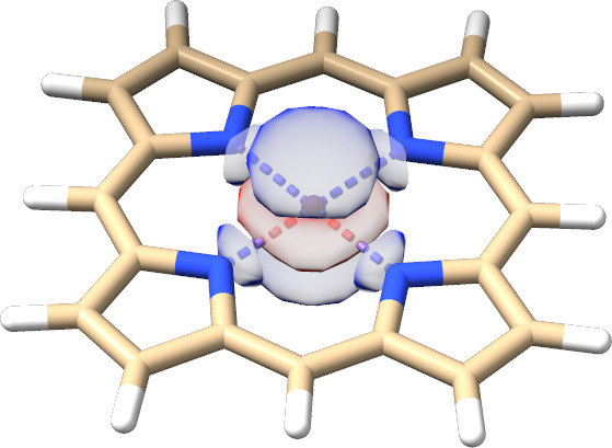AVAS LUMO

Fig. 6.13 Initial HOMO and LUMO AVAS orbitals of a bridged bithiophene biradical and FeTPP.

6.1.7.4. CASSCF and Symmetry

The CASSCF program can make some use of symmetry. Thus, it is possible to do the CI calculations separated by irreducible representations. This allows one to calculate electronic states in a more controlled fashion.

Let us look at a simple example: C\(_{2}\)H\(_{4}\). We first generate symmetry adapted MP2 natural orbitals. Since we opt for initial guess orbitals, the computationally cheaper unrelaxed density suffices:

! def2-TZVP def2-TZVP/C UseSym RI-MP2 conv # conventional is faster for small molecules
%mp2 
density unrelaxed
natorbs true 
end 
* int 0 1
C 0 0 0  0 0 0
C 1 0 0  1.35 0 0
H 1 2 0  1.1 120 0
H 1 2 3  1.1 120 180
H 2 1 3  1.1 120 0
H 2 1 3  1.1 120 180
*

The program does the following. It first identifies the group correctly as D\(_{2h}\) and sets up its irreducible representations. The process detects symmetry within SymThresh (\(10^{-4}\)) and purifies the geometry thereafter:

------------------
SYMMETRY DETECTION
------------------
The point group will now be determined using a tolerance of 1.0000e-04.
Splitting atom subsets according to nuclear charge, mass and basis set.
Splitting atom subsets according to distance from the molecule's center.
Identifying relative distance patterns of the atoms.
Splitting atom subsets according to atoms' relative distance patterns.
Bring atoms of each subset into input order.
The molecule is planar.
The molecule has a center of inversion.
Analyzing the first atom subset for its symmetry.
The atoms in the selected subset form a 4-gon with alternating side lengths.
Testing point group D2h.
Success!
This point group has been found:    D2h
Largest non-degenerate subgroup:    D2h


Symmetry-perfected Cartesians (point group D2h):

Atom          Symmetry-perfected Cartesians (x, y, z; au)
  0      -1.275565140397    0.000000000000    0.000000000000
  1       1.275565140397    0.000000000000    0.000000000000
  2      -2.314914514054    1.800205921988    0.000000000000
  3      -2.314914514054   -1.800205921988    0.000000000000
  4       2.314914514054    1.800205921988    0.000000000000
  5       2.314914514054   -1.800205921988    0.000000000000


-----------------------------------------------
SYMMETRY-PERFECTED CARTESIAN COORDINATES (A.U.)
-----------------------------------------------
Warning (ORCA_SYM): Coordinates were not cleaned so far!

------------------
SYMMETRY REDUCTION
------------------
ORCA supports only abelian point groups.
It is now checked, if the determined point group is supported:
Point Group ( D2h   ) is          ... supported

(Re)building abelian point group:
Creating Character Table          ... done
Making direct product table       ... done
Constructing symmetry operations  ... done
Creating atom transfer table      ... done
Creating asymmetric unit          ... done

----------------------
ASYMMETRIC UNIT IN D2h
----------------------
  #  AT     MASS              COORDS (A.U.)             BAS
   0 C   12.0110  -1.27556514   0.00000000   0.00000000   0
   2 H    1.0080  -2.31491451   1.80020592   0.00000000   0

----------------------
SYMMETRY ADAPTED BASIS
----------------------
The coefficients for the symmetry adapted linear combinations (SALCS)
of basis functions will now be computed:
Number of basis functions         ...    86
Preparing memory                  ... done
Constructing Gamma(red)           ... done
Reducing Gamma(red)               ... done
Constructing SALCs                ... done
Checking SALC integrity           ... nothing suspicious
Normalizing SALCs                 ... done

Storing the symmetry object:
Symmetry file                     ... Test-SYM-CAS-C2H4-1.sym.tmp
Writing symmetry information      ... done

It then performs the SCF calculation and keeps the symmetry in the molecular orbitals.

NO   OCC          E(Eh)            E(eV)    Irrep
   0   2.0000     -11.236728      -305.7669    1-Ag
   1   2.0000     -11.235157      -305.7242    1-B3u
   2   2.0000      -1.027144       -27.9500    2-Ag
   3   2.0000      -0.784021       -21.3343    2-B3u
   4   2.0000      -0.641566       -17.4579    1-B2u
   5   2.0000      -0.575842       -15.6694    3-Ag
   6   2.0000      -0.508313       -13.8319    1-B1g
   7   2.0000      -0.373406       -10.1609    1-B1u
   8   0.0000       0.139580         3.7982    1-B2g
   9   0.0000       0.171982         4.6799    4-Ag
  10   0.0000       0.195186         5.3113    3-B3u
  11   0.0000       0.196786         5.3548    2-B2u
  12   0.0000       0.242832         6.6078    2-B1g
  13   0.0000       0.300191         8.1686    5-Ag
  14   0.0000       0.326339         8.8801    4-B3u
... etc

The MP2 module does not take any advantage of this information but produces natural orbitals that are symmetry adapted:

N[  0](B3u) =   2.00000360
N[  1]( Ag) =   2.00000219
N[  2]( Ag) =   1.98056435
N[  3](B3u) =   1.97195041
N[  4](B2u) =   1.96746753
N[  5](B1g) =   1.96578954
N[  6]( Ag) =   1.95864726
N[  7](B1u) =   1.93107098
N[  8](B2g) =   0.04702701
N[  9](B3u) =   0.02071784
N[ 10](B2u) =   0.01727252
N[ 11]( Ag) =   0.01651489
N[ 12](B1g) =   0.01602695
N[ 13](B3u) =   0.01443373
N[ 14](B1u) =   0.01164204
N[ 15]( Ag) =   0.01008617
N[ 16](B2u) =   0.00999302
N[ 17]( Ag) =   0.00840326
N[ 18](B3g) =   0.00795053
N[ 19](B3u) =   0.00532044
N[ 20]( Au) =   0.00450556
etc.

From this information and visual inspection you will know what orbitals you will have in the active space:

These natural orbitals can then be fed into the CASSCF calculation. We perform a simple calculation in which we keep the ground state singlet (A\(_{1g}\) symmetry, irrep\(=\)0) and the first excited triplet state (B\(_{3u}\) symmetry, irrep\(=\)7). In general the ordering of irreps follows standard conventions and in case of doubt you will find the relevant number for each irrep in the output.

For example, here (using LargePrint):

----------------------------
CHARACTER TABLE OF GROUP D2h
----------------------------
GAMMA  O1   O2   O3   O4   O5   O6   O7   O8
 Ag :  1.0  1.0  1.0  1.0  1.0  1.0  1.0  1.0
 B1g:  1.0  1.0 -1.0 -1.0  1.0  1.0 -1.0 -1.0
 B2g:  1.0 -1.0  1.0 -1.0  1.0 -1.0  1.0 -1.0
 B3g:  1.0 -1.0 -1.0  1.0  1.0 -1.0 -1.0  1.0
 Au :  1.0  1.0  1.0  1.0 -1.0 -1.0 -1.0 -1.0
 B1u:  1.0  1.0 -1.0 -1.0 -1.0 -1.0  1.0  1.0
 B2u:  1.0 -1.0  1.0 -1.0 -1.0  1.0 -1.0  1.0
 B3u:  1.0 -1.0 -1.0  1.0 -1.0  1.0  1.0 -1.0

---------------------------------
DIRECT PRODUCT TABLE OF GROUP D2h
---------------------------------
   **   Ag  B1g B2g B3g Au  B1u B2u B3u

 Ag     Ag  B1g B2g B3g Au  B1u B2u B3u
 B1g    B1g Ag  B3g B2g B1u Au  B3u B2u
 B2g    B2g B3g Ag  B1g B2u B3u Au  B1u
 B3g    B3g B2g B1g Ag  B3u B2u B1u Au
 Au     Au  B1u B2u B3u Ag  B1g B2g B3g
 B1u    B1u Au  B3u B2u B1g Ag  B3g B2g
 B2u    B2u B3u Au  B1u B2g B3g Ag  B1g
 B3u    B3u B2u B1u Au  B3g B2g B1g Ag

We use the following input for CASSCF, where we tightened the integral cut-offs and the convergence criteria using !VeryTightSCF.

! def2-TZVP  Conv NormalPrint UseSym
! moread
%moinp "Test-SYM-CAS-C2H4-1.mp2nat"
%casscf nel            4 
        norb           4
        # This is only here to show that NR can also be used from 
        # the start with orbstep 
        orbstep    nr
        switchstep nr
        # the lowest singet and triplet states. The new feature 
        # is the array "irrep" that lets you give the irrep for 
        # a given block. Thus, now you can have several blocks of
        # the same multiplicity but different spatial symmetry
        irrep       0,7
        mult        1,3
        nroots      1,1
        end

* int 0 1
C 0 0 0  0 0 0
C 1 0 0  1.35 0 0
H 1 2 0  1.1 120 0
H 1 2 3  1.1 120 180
H 2 1 3  1.1 120 0
H 2 1 3  1.1 120 180
*

And gives:

------------
SCF SETTINGS
------------
Hamiltonian:
 Ab initio Hamiltonian  Method          .... Hartree-Fock(GTOs)


General Settings:
 Integral files         IntName         .... Test-SYM-CAS-C2H4-1
 Hartree-Fock type      HFTyp           .... CASSCF
 Total Charge           Charge          ....    0
 Multiplicity           Mult            ....    1
 Number of Electrons    NEL             ....   16
 Basis Dimension        Dim             ....   86
 Nuclear Repulsion      ENuc            ....     32.9609050695 Eh

 Symmetry handling      UseSym         .... ON
 Point group                           .... D2h
 Used point group                      .... D2h
 Number of irreps                      .... 8
   Irrep   Ag has   19 symmetry adapted basis functions (ofs=   0)
   Irrep  B1g has   12 symmetry adapted basis functions (ofs=  19)
   Irrep  B2g has    8 symmetry adapted basis functions (ofs=  31)
   Irrep  B3g has    4 symmetry adapted basis functions (ofs=  39)
   Irrep   Au has    4 symmetry adapted basis functions (ofs=  43)
   Irrep  B1u has    8 symmetry adapted basis functions (ofs=  47)
   Irrep  B2u has   12 symmetry adapted basis functions (ofs=  55)
   Irrep  B3u has   19 symmetry adapted basis functions (ofs=  67)

And further in the CASSCF program:

Symmetry handling      UseSym     ... ON
Point group                       ... D2h
Used point group                  ... D2h
Number of irreps                  ... 8
   Irrep   Ag has   19 SALCs (ofs=   0) #(closed)=   2 #(active)=   1
   Irrep  B1g has   12 SALCs (ofs=  19) #(closed)=   1 #(active)=   0
   Irrep  B2g has    8 SALCs (ofs=  31) #(closed)=   0 #(active)=   1
   Irrep  B3g has    4 SALCs (ofs=  39) #(closed)=   0 #(active)=   0
   Irrep   Au has    4 SALCs (ofs=  43) #(closed)=   0 #(active)=   0
   Irrep  B1u has    8 SALCs (ofs=  47) #(closed)=   0 #(active)=   1
   Irrep  B2u has   12 SALCs (ofs=  55) #(closed)=   1 #(active)=   0
   Irrep  B3u has   19 SALCs (ofs=  67) #(closed)=   2 #(active)=   1
 Symmetries of active orbitals:
   MO =    6  IRREP= 0 (Ag)
   MO =    7  IRREP= 5 (B1u)
   MO =    8  IRREP= 2 (B2g)
   MO =    9  IRREP= 7 (B3u)

Setting up the integral package       ... done
Building the CAS space                ... done (7 configurations for Mult=1 Irrep=0)
Building the CAS space                ... done (4 configurations for Mult=3 Irrep=7)

Note that the irrep occupations and active space irreps will be frozen to what they are upon entering the CASSCF program. This helps to setup the CI problem.

After which it smoothly converges to give:

    6:  1.986258       -0.753012    -20.4905   3-Ag
    7:  1.457849       -0.291201     -7.9240   1-B1u
    8:  0.541977        0.100890      2.7454   1-B2g
    9:  0.013915        0.964186     26.2368   3-B3u

As well as:

-----------------------------
SA-CASSCF TRANSITION ENERGIES
------------------------------

LOWEST ROOT =    -78.110314788 Eh -2125.490 eV

STATE   ROOT MULT IRREP DE/a.u.    DE/eV    DE/cm**-1
   1:    0    3  B3u   0.163741     4.456  35937.1

6.1.7.5. RI, RIJCOSX and RIJK approximations for CASSCF

A significant speedup of CASSCF calculations on larger molecules can be achieved with the RI, RI-JK and RIJCOSX approximations. [459] There are two independent integral generation and transformation steps in a CASSCF procedure. In addition to the usual Fock matrix construction, that is central to HF and DFT approaches, more integrals appear in the construction of the orbital gradient and Hessian. The latter are approximated using the keyword trafostep RI, where an auxiliary basis (/C or the more accurate /JK auxiliary basis) is required. Note that auxiliary basis sets of the type /J are not sufficient to fit these integrals. If no suitable auxiliary basis set is available, the AutoAux feature might be useful (see comment in the input below). [827] We note passing, that there are in principle three distinguished auxiliary basis slots, that can be individually assigned in the %basis block (section Choice of Basis Set). As an example, we recompute the benzene ground state example from Section Starting Orbitals with a CAS(6,6).

! SV(P) def2-svp/C
! moread
%moinp "Test-CASSCF-Benzene-2.mrci.nat"

# Commented out: Detailed settings of the auxiliary basis in the %basis block,
#                where the AuxC slot is relevant for the option TrafoStep RI.                
# %basis 
# auxC "def2-svp/C" # "AutoAux" or "def2/JK"
# end

%casscf  nel    6
         norb   6
         nroots 1
         mult   1         
         trafostep ri
         end

The energy of this calculation is -230.590328 Eh compared to the previous result -230.590271 Eh. Thus, the RI error is only 0.06 mEh which is certainly negligible for all intents and purposes. With the larger /JK auxiliary basis the error is typically much smaller (0.02 mEh in this example). Even if more accurate results are necessary, it is a good idea to pre-converge the CASSCF with RI. The resulting orbitals should be a much better guess for the subsequent calculation without RI and thus save computation time.

The TrafoStep RI only affects the integral transformation in CASSCF calculations while the Fock operators are still calculated in the standard way using four index integrals. In order to fully avoid any four-index integral evaluation, you can significantly speed up the time needed in each iteration by specifying !RIJCOSX. The keyword implies TrafoStep RI . The COSX approximation is used for the construction of the Fock matrices. In this case, an additional auxiliary basis (/J auxiliary basis) is mandatory.

! SV(P) def2-svp/C RIJCOSX def2/J
! moread
%moinp "Test-CASSCF-Benzene-2.mrci.nat"

# Commented out: Detailed settings of the auxiliary basis in the %basis block,
#                where the AuxJ and AuxC slot are mandatory.
# %basis 
# auxJ "def2/J"     # "AutoAux"
# auxC "def2-svp/C" # "AutoAux", "def2/JK"
# end

%casscf  nel    6
  norb   6
  nroots 1
  mult   1
end

The speedup and accuracy is similar to what is observed in RHF and UHF calculations. In this example the RIJCOSX leads to an error of 1 mEh. The methodology performs better for the computation of energy differences, where it profits from error cancellation. The RIJCOSX is ideally suited to converge large-scale systems. Note that for large calculations the integral cut-offs and numerical grids should be tightened. See section Using the RI Approximation for Hartree-Fock and Hybrid DFT (RIJCOSX) for details. With a floppy numerical grid setting the accuracy as well as the convergence behavior of CASSCF deteriorate. The RIJK approximation offers an alternative ansatz. The latter is set with !RIJK and can also be run in conventional mode (conv) for additional speed-up. With conv, a single auxiliary basis must be provided that is sufficiently larger to approximate the Fock matrices as well the gradient/Hessian integrals. In direct mode an additional auxiliary basis set can be set for the AuxC slot.

! SV(P) RIJK  def2/JK

# Commented out: Detailed settings of the auxiliary basis in the %basis block,
#                where only the auxJK slot must be set.
# %basis 
# auxJK "def2/JK" # or "AutoAux"
# end

The RIJK methodology is more accurate and robust for CASSCF e.g. here the error is just 0.5 mEH.

Organic molecules with nearly double occupied orbitals can be challenge for the orbital optimization process. We compare calculations done with/without the NR solver:

! SV(P)
! moread
%moinp "Test-CASSCF-Benzene-2.mrci.nat"

%casscf  nel    6
  norb   6
  nroots 1
  mult   1
  # overwriting default settings with NR close to convergence
  switchstep NR 
end

The NR variant takes 5 cycles to converge, whereas the default (SuperCI_PT) requires 8 cycles. In general, first order methods, take more iterations compared to the NR method. However, first order methods are much cheaper than the NR and therefore it may pay off to do a few iterations more rather than switching to the expensive second order methods. Moreover, second order methods are less robust and may diverge in certain circumstances (too far from convergence). When playing with the convergence settings, there is always a trade-off between speed versus robustness. The default settings are chosen carefully.[459] Facing convergence problems, it can be useful to use an alternative scheme (orbstep SuperCI and switchstep DIIS) in conjunction with a level-shifts (ShiftUp, ShiftDn). Alternatively, changing the guess orbitals may avoid convergence problems as well.

6.1.7.6. Robust Convergence with TRAH-CASSCF

The restricted-step second-order converger TRAH Quadratic Convergence is now also available for both state-specific and state-averaged CASSCF calculations.[382] To activate TRAH for your CASSCF calculation, you just need to add !TRAH in one of the simple input lines and add an auxiliary basis.

! TRAH Def2-SVP Def2-SVP/C TightSCF

%casscf
  nel 6
  norb 6
  mult 1
  nroots 2
end

*xyz 0 1
  N   0.0   0.0   0.0
  N   0.0   0.0   1.1
end

In most cases, there is no need to play with any input parameters. The only exception is the choice of active molecular orbital representations that can have a significant impact on the convergence rate for spin-coupled systems. As can be seen from Fig. Fig. 6.14, for such calculations localized active orbitals perform best. In any other case, the natural orbitals (default) should be employed.

Fig. 6.14 SXPT and TRAH error convergence using different choices for the active-orbital basis.

Possible input options for the active-orbital basis are

%casscf
 TRAHCAS
  #ActiveMOs NotSet
  #ActiveMOs Canonical
  #ActiveMOs Localized
  ActiveMOs Natural   # default
 end
end

Active Orbitals	Meaning
Natural	Keeps the one-electron density matrix (1-RDM) diagonal. Default
Localized	A Foster-Boys localization of active MOs is performed in every macro iteration.
	This is recommended for spin-coupled systems.
NotSet	The active MO basis is not changed. Primarily debug option.
Canonical	Keeps the total active-MO Fock matrix diagonal. Experimental option.

Note that, in contrast to the SCF program, there is no AutoTRAH feature for CASSCF yet. The TRAH feature has to be requested explicitly in the input.

6.1.7.7. Breaking Chemical Bonds

Let us turn to the breaking of chemical bonds. As a first example we study the dissociation of the H\(_{2}\) molecule. Scanning a bond, we have two potential setups for the calculation: a) scan from the inside to the outside or b) from the outside to inside. Of course both setups yield identical results, but they differ in practical aspects i.e. convergence properties. In general, scanning from the outside to the inside is the recommended procedure. Using the default guess (PModel), starting orbitals are much easier identified than at shorter distances, where the antibonding orbitals are probably ‘impure’ and hence would require some additional preparation. To ensure a smooth potential energy surface, in all subsequent geometry steps, ORCA reads the converged CASSCF orbitals from the previous geometry step. In the following, TightSCF is used to tighten the convergence settings of CASSCF.

!Def2-SVP TightSCF 

%casscf
 nel         2   
 norb        2   
 mult        1   
 nroots      1   
end

# Scanning from the outside to the inside
%paras 
 R [4.1 3.8 3.5 3.2 2.9 2.6 2.4 2.2 
    2 1.7 1.5 1.3 1.1 1 0.9 0.8 
    0.75 0.7 0.65 0.6]
end

* xyz 0 1 
 H   0.0   0.0   0.0 
 H   0.0   0.0   {R} 
end

The resulting potential energy surface (PES) is depicted in Fig. 6.15 together with PESs obtained from RHF and broken-symmetry UHF calculations (input below).

! RHF Def2-SVP TightSCF

# etc...

And

! UHF Def2-SVP TightSCF

%scf
  FlipSpin 1
  FinalMs 0.0
end

# etc...

Note

The FlipSpin option does not work together with the parameter scan. Only the first structure will undergo a spin flip. Therefore, at the current status, a separate input file (including the coordinates or with a corresponding coordinate file) has to be provided for each structure that is scanned along the PES.

Fig. 6.15 Potential Energy Surface of the H\(_2\) molecule from RHF, UHF and CASSCF(2,2) calculations (Def2-SVP basis).

It is obvious, that the CASSCF surface is concise and yields the correct dissociation behavior. The RHF surface is roughly parallel to the CASSCF surface in the vicinity of the minimum but then starts to fail badly as the H-H bond starts to break. The broken-symmetry UHF solution is identical to RHF in the vicinity of the minimum and dissociates correctly. It is, however, of rather mediocre quality in the intermediate region where it follows the RHF surface.

A more challenging case is to dissociate the N-N bond of the N\(_{2}\) molecule correctly. Using CASSCF with the six p-orbitals we get a nice potential energy curve (The depth of the minimum is still too shallow compared to experiment by some 1 eV or so. A good dissociation energy requires a dynamic correlation treatment on top of CASSCF and a larger basis set).

Fig. 6.16 Potential Energy Surface of the N\(_2\) molecule from CASSCF(6,6) calculations (Def2-SVP basis).

One can use the H\(_{2}\) example to illustrate the state-averaging feature. Since we have two active electrons we have two singlets and one triplet. Let us average the orbitals over these three states (we take equal weights for all multiplicity blocks):

!Def2-SVP TightSCF 

%casscf
 nel         2   
 norb        2   
 mult        3,1 
 nroots      1,2 
end

# Scanning from the outside to the inside
%paras 
R [4.1 3.8 3.5 3.2 2.9 2.6 2.4 2.2 
   2 1.7 1.5 1.3 1.1 1 0.9 0.8 
   0.75 0.7 0.65 0.6]
end

* xyz 0 1 
 H 0 0 0 
 H 0 0 {R} 
end

which gives:

Fig. 6.17 State averaged CASSCF(2,2) calculations on H\(_2\) (two singlets, one triplet; Def2-SVP basis). The grey curve is the ground state CASSCF(2,2) curve

One observes, that the singlet and triplet ground states become degenerate for large distances (as required) while the second singlet becomes the ionic singlet state which is high in energy. If one compares the lowest root of the state-averaged calculation (in green) with the dedicated ground state calculation (in gray) one gets an idea of the energetic penalty that is associated with averaged as opposed to dedicated orbitals.

A more involved example is the rotation around the double bond in C\(_{2}\)H\(_{4}\). Here, the \(\pi\)-bond is broken as one twists the molecule. The means the proper active space consists of two active electron in two orbitals.

The input is (for fun, we average over the lowest two singlets and the triplet):

!def2-SVP TightSCF

%casscf 
 nel        2   
 norb       2   
 mult       3,1 
 nroots     1,2 
end

%paras
 Alpha = 0,180,37
end

* int 0 1 
 C  0  0  0  0      0   0   
 C  1  0  0 1.34    0   0   
 H  1  2  0 1.07  120   0   
 H  1  2  3 1.07  120 180 
 H  2  1  3 1.07  120 {Alpha}
 H  2  1  3 1.07  120 {Alpha+180}
edn

Fig. 6.18 State averaged CASSCF(2,2) calculations on C\(_2\)H\(_4\) (two singlets, one triplet; SV(P) basis). The grey curve is the state averaged energy.

We can see from this plot, that the CASSCF method produces a nice ground state surface with the correct periodicity and degeneracy at the end points, which represent the planar ethylene molecule. At 90\(^{\circ}\) one has a weakly coupled diradical and the singlet and triplet states become nearly degenerate, again as expected. Calculations with larger basis sets and inclusion of dynamic correlation would give nice quantitative results.

6.1.7.8. Excited States

As a final example, we do a state-average calculation on H\(_{2}\)CO in order to illustrate excited state treatments. We expect from the ground state (basically closed-shell) a n \(\to \pi^{\ast }\) and a \(\pi \to \pi^{\ast }\) excited state which we want to describe. For the n\(\to \pi^{\ast }\) we also want to calculate the triplet since it is well known experimentally. First we take DFT orbitals as starting guess.

! BP86 Def2-SVP TightSCF

*int 0 1
 C  0 0 0 0.00   0.0    0.00
 O  1 0 0 1.20   0.0    0.00
 H  1 2 0 1.10 120.0    0.00
 H  1 2 3 1.10 120.0  180.00
end

In this example the DFT calculation produces the desired active space (n,\(\pi\) and\(\pi^\ast\) orbitals) without further modification (e.g. swapping orbitals). In general it is advised to verify the final converged orbitals.

! Def2-SVP TightSCF MOREAD

%moinp "orbs.gbw"

%casscf 
 nel         4 
 norb        3 
 mult        1,3
 nroots      3,1
end

*int 0 1
C  0 0 0 0.00   0.0    0.00
O  1 0 0 1.20   0.0    0.00
H  1 2 0 1.10 120.0    0.00
H  1 2 3 1.10 120.0  180.00
end

We get:

-----------------------------
SA-CASSCF TRANSITION ENERGIES
------------------------------

LOWEST ROOT (ROOT 0 ,MULT 1) =   -113.805194041 Eh -3096.797 eV

STATE   ROOT MULT  DE/a.u.    DE/eV    DE/cm**-1
1:    0    3   0.129029     3.511  28318.5
2:    1    1   0.141507     3.851  31057.3
3:    2    1   0.453905    12.351  99620.7

The triplet n \(\to \pi^{\ast }\) states is spot on with the experiment excitation energy of 3.5 eV.[725] Similarly, the singlet n \(\to \pi^{\ast }\) excited state is well reproduced compared to 3.79 eV and 4.07 eV reported in the literature.[725, 878] Only the singlet \(\pi \to \pi^{\ast }\) excited state stands out compared to the theoretical estimate of 9.84 eV computed with MR-AQCC.[542]. The good results are very fortuitous given the small basis set, the minimal active space and the complete neglect of dynamical correlation.

The state-average procedure might not do justice to the different nature of the states (n \(\to \pi^{\ast }\) versus \(\pi \to \pi^{\ast }\)). The agreement should be better with the orbitals optimized for each state. In ORCA, state-specific optimization are realized adjusting the weights i.e. for the second singlet excited root:

Second-Singlet:
%casscf 
  nel         4
  norb        3
  mult        1
  nroots      3
  weights[0] = 0,0,1 # weights for the roots
end

Note, that state-specific orbital optimization are challenging to converge and often prone to root-flipping.[511]

To analyze electronic transitions, natural transition orbitals (NTO) are available for state-averaged CASSCF (and also CASCI) calculations. NTOs are switched on for every ground- to excited-state transition by just adding DoNTO true to the %casscf ... end input block, i.e.

%casscf
  nel    4
  norb   3
  mult   1,3
  nroots 3,1
  DoNTO  true
end

For each excitation, the most dominant natural occupation numbers (singular values >1.e-4) are printed for each transition. A set of donor orbitals and a set of acceptor orbitals, each of dimension N_bf x (N_occ + N_act), are created and stored in files with unique names. We obtain for the previous formamide example the following CASSCF NTO output

==========================================
CASSCF Natural Transition Orbitals
==========================================

------------------------------------------------
NATURAL TRANSITION ORBITALS FOR STATE     1 1A  
------------------------------------------------

STATE    1 1A  :  E=   0.141508 au      3.851 eV    31057.3 cm**-1

Threshold for printing occupation numbers 1.0000e-04

     0  : n=  1.30882812
     1  : n=  0.02641080

=> Natural Transition Orbitals (donor   ) were saved in Test-CASSCF.H2CO-1.casscf.1-1A_nto-donor.gbw
=> Natural Transition Orbitals (acceptor) were saved in Test-CASSCF.H2CO-1.casscf.1-1A_nto-acceptor.gbw

------------------------------------------------
NATURAL TRANSITION ORBITALS FOR STATE     2 1A  
------------------------------------------------

STATE    2 1A  :  E=   0.453905 au     12.351 eV    99620.7 cm**-1

Threshold for printing occupation numbers 1.0000e-04

     0  : n=  1.30519478
     1  : n=  0.24869813
     2  : n=  0.00471742

=> Natural Transition Orbitals (donor   ) were saved in Test-CASSCF.H2CO-1.casscf.2-1A_nto-donor.gbw
=> Natural Transition Orbitals (acceptor) were saved in Test-CASSCF.H2CO-1.casscf.2-1A_nto-acceptor.gbw

For each transition, plots of the NTO pairs can be generated with the orca_plot program (see Sec. Orbital and Density Plots for details), e.g. acceptor orbitals of the 2 ¹A₁ state in interactive mode:

orca_plot Test-CASSCF.H2CO-1.casscf.2-1A_nto-acceptor.gbw -i

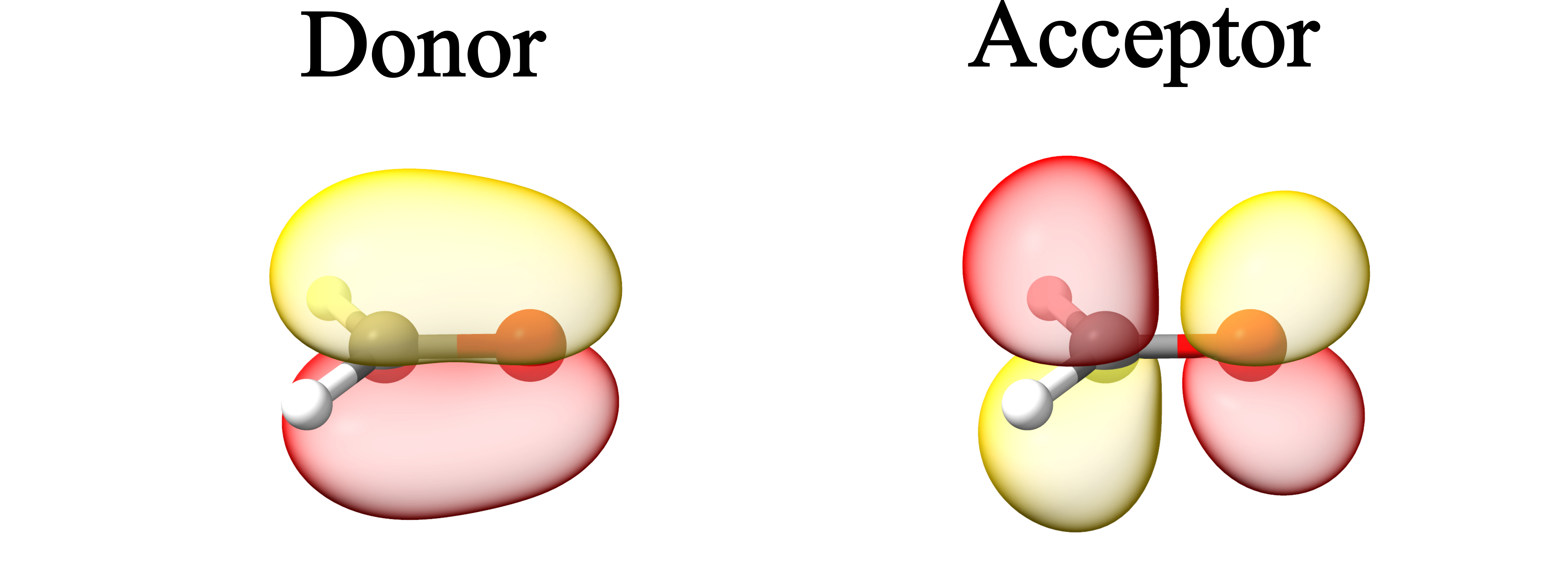
Fig. 6.19 Most dominant natural transition orbital (NTO) pair for the 2 ¹A₁ (S₂) transition in formaldehyde.

Alternatively, NTOs can also be computed directly in orca_plot from the CASSCF transition density matrices. Those need to be stored and kept in the density container by invoking

! KeepTransDensity

6.1.7.9. CASSCF Natural Orbitals as Input for Coupled-Cluster Calculations

Consider the possibility that you are not sure about the orbital occupancy of your system. Hence you carry out some CASSCF calculation for various states of the system in an effort to decide on the ground state. You can of course follow the CASSCF by MR-MP2 or MR-ACPF or SORCI calculations to get a true multireference result for the state ordering. Yet, in some cases you may also want to obtain a coupled-cluster estimate for the state energy difference. Converging coupled-cluster calculation on alternative states in a controlled manner is anything but trivial. Here a feature of ORCA might be helpful. The best single configuration that resembles a given CASSCF state is built from the natural orbitals of this state. These orbitals are also ordered in the right way to be input into the MDCI program. The convergence to excited states is, of course, not without pitfalls and limitations as will become evident in the two examples below.

As an example, consider some ionized states of the water cation:

First, we generate the natural orbitals for each state with the help of the MRCI module. To this end we run a state average CASSCF for the lowest three doublet states and pass that information on to the MRCI module that does a CASCI calculation and produces the natural orbitals:

! ano-pVDZ TightSCF

%casscf  
 nel     7   
 norb    6   
 nroots  3
 mult    2   
end

%mrci    
 tsel       0   
 tpre       0   
 donatorbs  2
 densities  5,1 
 newblock 2 * 
  nroots 3 
  excitations none 
  refs 
   cas(7,6)
  end 
 end 
end

* int 1 2 
 O     0   0   0   0.000000     0.000     0.000
 H     1   0   0   1.012277     0.000     0.000
 H     1   2   0   1.012177   109.288     0.000
end

This produces the files Basename.bm_sn.nat where “m” is the number of the block (m = 0 correspond to the doublet in this case) and “n” stands of the relevant state (n = 0,1,2).

These natural orbitals are then fed into unrestricted QCISD(T) calculations:

! ano-pVDZ TightSCF QCISD(T) MOREAD NoIter

%moinp "H2O+.b0_s0.nat"

* int 1 2
 O     0   0   0   0.000000     0.000     0.000
 H     1   0   0   1.012277     0.000     0.000
 H     1   2   0   1.012177   109.288     0.000
*

As a reference we also perform a SORCI on the same system

! ano-pVDZ TightSCF SORCI

%casscf
 nel     7
 norb    6
 nroots  3
 mult    2
end

* int 1 2
 O     0   0   0   0.000000     0.000     0.000
 H     1   0   0   1.012277     0.000     0.000
 H     1   2   0   1.012177   109.288     0.000
*

we obtain the transition energies:

      SORCI   QCISD(T) (in cm-1)
  D0      0     0.0
  D1  16269   16293
  D2  50403   50509

Thus, in this example the agreement between single- and multireference methods is good and the unrestricted QCISD(T) method is able to describe these excited doublet states. The natural orbitals have been a reliable way to guide the CC equations into the desired solutions. This will work in many cases.

6.1.7.10. Large Scale CAS-SCF calculations using ICE-CI

The CASSCF procedure can be used for the calculation of spin-state energetics of molecules showing a multi-reference character via the state-averaged CASSCF protocol as described in the CASSCF section The Complete Active Space Self-Consistent Field (CASSCF) Module. The main obstacle in getting qualitatively accurate spin-state energetics for molecules with many transition metal centers is the proper treatment of the static-correlation effects between the large number of open-shell electrons. In this section, we describe how one can effectively perform CASSCF calculations on such systems containing a large number of high-spin open-shell transition metal atoms.

As an example, consider the Iron-Sulfur dimer \([\text{Fe(III)}_2\text{SR}_2]^2-\) molecule. In this system, the Fe(III) centers can be seen as being made up mostly of S=5/2 local spin states (lower spin states such as 3/2 and 1/2 will have small contributions due to Hunds’ rule.) The main hurdle while using the CASSCF protocol on such systems (with increasing number of metal atoms) is the exponential growth of the Hilbert space although the physics can be effectively seen as occurring in a very small set of configuration state functions (CSFs). Therefore, in order to obtain qualitatively correct spin-state energetics, one need not perform a Full-CI on such molecules but rather a CIPSI like procedure using the ICE-CI solver should give chemically accurate results. In the case of the Fe(III) dimer, one can imagine that the ground singlet state is composed almost entirely of the CSF where the two Fe(III) centers are coupled antiferromagnetically. Such a CSF is represented as follows:

\[\left| \Psi_0^{S=0} \right\rangle= \left[ 1, 1, 1, 1, 1, -1, -1, -1, -1, -1 \right]\]

In order to make sense of this CSF representation, one needs to clarify a few points which are as follows:

• First, in the above basis the 10 orbitals are localized to 5 on each Fe center (following a high-spin UHF/UKS calculation.)

• Second, the orbitals are ordered (as automatically done in ORCA_LOC) such that the first five orbitals lie on one Fe(III) center and the last five orbitals on the second Fe(III) center.

Using this ordering, one can read the CSF shown above in the following way: The first five 1 represent the five electrons on the first Fe(III) coupled in a parallel fashion to give a S=5/2 spin. The next five -1 represent two points:

• First, the five consecutive -1 signify the presence of five ferromagnetically coupled electrons on the second Fe(III) center resulting in a local S=5/2 spin state.

• Second, the second set of spins are coupled to the first 1 via anti-parallel coupling as signified by the sign of the last five -1 entries.

Therefore, we can see that using the CSF representation, one can obtain an extremely compact representation of the wavefunction for molecules consisting of open-shell transition metal atoms. This protocol of using localized orbitals in a specified order to form compact CSF representations for transition metal systems can be systematically extended for large molecules.

We will use the example of the Iron-Sulfur dimer \([\text{Fe(III)}_2\text{SR}_2]^2-\) to demonstrate how to prepare a reference CSF and perform spin-state energetics using the state-averaged CASSCF protocol. In such systems, often one can obtain an estimate of the energy gap between the singlet-state and the high-spin states from experiment. Ab initio values for this gap be obtained using the state-averaged CASSCF protocol using the input shown below.

! def2-SVP MOREAD
 
%moinp "locorbs.gbw"

%casscf 
 nel     10
 norb    10
 mult    11,1
 nroots  1,1
 refs                              # reference for multiplicity 11
  { 1 1 1 1 1  1  1  1  1  1}
 end
 refs                              # reference for multiplicity 1
  { 1 1 1 1 1 -1 -1 -1 -1 -1}
 end
  cistep ice
 ci
  icetype 1
 end
 actorbs unchanged
end

* xyz -2 11
Fe          0.000000000      0.000000000     -1.343567812
Fe          0.000000000      0.000000000      1.343567812
S           1.071733501      1.373366082      0.000000000
S           1.346714284     -1.345901486     -2.651621449
S          -1.346714284      1.345901486     -2.651621449
S          -1.071733501     -1.373366082      0.000000000
S          -1.346714284      1.345901486      2.651621449
S           1.346714284     -1.345901486      2.651621449
C          -2.485663304      0.362543393     -3.600795276
H          -3.319937516      0.596731755     -3.505882795
H          -2.347446507      0.388292903     -4.463380590
H          -2.472404709     -0.485711203     -3.404167343
C           2.485663304     -0.362543393     -3.600795276
H           3.319937516     -0.596731755     -3.505882795
H           2.347446507     -0.388292903     -4.463380590
H           2.472404709      0.485711203     -3.404167343
C           2.485663304     -0.362543393      3.600795276
H           2.347446507     -0.388292903      4.463380590
H           3.319937516     -0.596731755      3.505882795
H           2.472404709      0.485711203      3.404167343
C          -2.485663304      0.362543393      3.600795276
H          -3.319937516      0.596731755      3.505882795
H          -2.472404709     -0.485711203      3.404167343
H          -2.347446507      0.388292903      4.463380590
*

The main keyword that needs to be used here (unlike in other CAS-SCF calculations) is the actorbs keyword. Since we are using a local basis with a specific ordering of the orbitals, in order to represent our wavefunction it is imperative to preserve the local nature of the orbitals as well as the orbital ordering. Therefore, we do not calculate natural orbitals at the end of the CASSCF calculation (as is traditionally done) instead we impose the orbitals to be as similar to the input orbitals as possible. This is automatically enabled for intermediate CASSCF macro iterations. The resulting CASSCF calculation provides a chemically intuitive and simple wavefunction and transition energy as shown below:

---------------------------------------------
CAS-SCF STATES FOR BLOCK  1 MULT=11 NROOTS= 1
---------------------------------------------

STATE   0 MULT=11: E=  -5066.8462457411 Eh W=  0.5000 DE= 0.000 eV      0.0 cm**-1
      1.00000 ( 1.000000000) CSF = 1+1+1+1+1+1+1+1+1+1+



---------------------------------------------
CAS-SCF STATES FOR BLOCK  2 MULT= 1 NROOTS= 1
---------------------------------------------

STATE   0 MULT= 1: E=  -5066.8548894831 Eh W=  0.5000 DE= 0.000 eV      0.0 cm**-1
      0.98159 (-0.990753235) CSF = 1+1+1+1+1+1-1-1-1-1-



-----------------------------
SA-CASSCF TRANSITION ENERGIES
------------------------------

LOWEST ROOT (ROOT 0 ,MULT 1) =  -5066.854889483 Eh -137876.131 eV

STATE   ROOT MULT  DE/a.u.    DE/eV    DE/cm**-1
   1:    0   11   0.008644     0.235   1897.1

As we can see from the output above, 98% of the wavefunction for the singlet-state is given by a single CSF which we gave as a reference CSF. This CSF has a very simple chemical interpretation representing the anti-parallel coupling between the two high-spin Fe(III) centers. Since Iron-Sulfur molecules show a strong anti-ferromagnetic coupling, we expect the singlet state to be lower in energy than the high-spin (S=5) state. The CASSCF transition energies show essentially this fact. The transition energy is about \(\text{2000cm}^{-1}\) which is what one expects from a CASSCF calculation on such sulfide bridged transition-metal molecules.

6.1.8. N-Electron Valence State Perturbation Theory (NEVPT2)

NEVPT2 is an internally contracted multireference perturbation theory, which applies to CASSCF type wavefunctions. The NEVPT2 method, as described in the original papers of Angeli et al, comes in two flavor the strongly contracted NEVPT2 (SC-NEVPT2) and the so called partially contracted NEVPT2 (PC-NEVPT2).[44, 45, 46] In fact, the latter employs a fully internally contracted wavefunction and should more appropriately called FIC-NEVPT2. Both methods produces energies of similar quality as the CASPT2 approach.[366, 756] The strongly and fully internally contracted NEVPT2 are implemented in ORCA together with a number of approximations that makes the methodology very attractive for large scale applications. In conjunction with the RI approximation systems with active space of to 16 active orbitals and 2000 basis functions can be computed. With the newly developed DLPNO version of the FIC-NEVPT2 the size of the molecules does not matter anymore.[344] For a more complete list of keywords and features, we refer to detailed documentation section N-Electron Valence State Pertubation Theory.

Besides corrections to the correlation energy, ORCA features UV, IR, CD and MCD spectra as well as EPR parameters for NEVPT2. These properties are computed using the “quasi-degenerate perturbation theory” that is described in section CASSCF Properties. The NEVPT2 corrections enter as “improved diagonal energies” in this formalism. ORCA also features the multi-state extension (QD-NEVPT2) for the strongly contracted NEVPT2 variant.[48, 493] Here, the reference wavefunction is revised in the presence of dynamical correlation. For systems, where such reference relaxation is important, the computed spectroscopic properties will improve.

As a simple example for NEVPT2, consider the ground state of the nitrogen molecule N\(_{2}\) . After defining the computational details of our CASSCF calculation, we insert “!SC-NEVPT2” as simple input or specify “PTMethod SC_NEVPT2” in the %casscf block. Please note the difference in the two keywords’ spelling: Simple input uses hyphen, block input uses underscore for technical reasons. There are more optional settings, which are described in section N-Electron Valence State Pertubation Theory of this manual.

!def2-svp nofrozencore PAtom
%casscf nel  6
        norb 6
        mult 1
        PTMethod SC_NEVPT2  # SC_NEVPT2   for strongly contracted NEVPT2
                            # FIC_NEVPT2  for the fully internally contracted NEVPT2
                            # DLPNO_NEVPT2 for the FIC-NEVPT2 with DLPNO
                            # DLPNO requires: trafostep RI and an aux basis
end

* xyz 0 1
N	0.0	0.0	0.0
N	0.0	0.0	1.09768
*

For better control of the program flow it is advised to split the calculation into two parts. First converge the CASSCF wave function and then in a second step read the converged orbitals and execute the actual NEVPT2.

---------------------------------------------------------------
                        ORCA-CASSCF
---------------------------------------------------------------

...
PT2-SETTINGS:
A PT2 calculation will be performed on top of the CASSCF wave function (PT2 = SC-NEVPT2)
...
---------------------------------------------------------------
                         < NEVPT2  >
---------------------------------------------------------------
...
 ===============================================================
                       NEVPT2 Results
===============================================================
   *********************
    MULT 1, ROOT 0
   *********************

  Class V0_ijab :        dE = -0.017748
  Class Vm1_iab :        dE = -0.023171
  Class Vm2_ab  :        dE = -0.042194
  Class V1_ija  :        dE = -0.006806
  Class V2_ij   :        dE = -0.005056
  Class V0_ia   :        dE = -0.054000
  Class Vm1_a   :        dE = -0.007091
  Class V1_i    :        dE = -0.001963

---------------------------------------------------------------
         Total Energy Correction : dE = -0.15802909
---------------------------------------------------------------
         Zero Order Energy       : E0 = -108.98888640
---------------------------------------------------------------
         Total Energy (E0+dE)    : E  = -109.14691549
---------------------------------------------------------------

Introducing dynamic correlation with the SC-NEVPT2 approach lowers the energy by 150 mEh. ORCA also prints the contribution of each “excitation class V” to the first order wave function. We note that in the case of a single reference wavefunction corresponding to a CAS(0,0) the V0_ij,ab excitation class produces the exact MP2 correlation energy. Unlike older versions of ORCA (pre version 4.0), NEVPT2 calculations employ the frozen core approximation by default. Results from previous versions can be obtained with the added keyword !NoFrozenCore.

In chapter Breaking Chemical Bonds the dissociation of the N\(_{2}\) molecule has been investigated with the CASSCF method. Inserting PTMethod SC_NEVPT2 into the %casscf block we obtain the NEVPT2 correction as additional information.

! def2-svp nofrozencore 
%casscf nel  6
        norb 6
        mult 1
        PTMethod SC_NEVPT2
end

# scanning from the outside to the inside
%paras
	R = 2.5,0.7, 30
end

*xyz 0 1
N 0.0 0.0 0.0
N 0.0 0.0 {R}
*

Fig. 6.20 Potential Energy Surface of the N\(_2\) molecule from CASSCF(6,6) and NEVPT2 calculations (def2-SVP).

All of the options available in CASSCF can in principle be applied to NEVPT2. Since NEVPT2 is implemented as a submodule of CASSCF, it will inherit all settings from CASSCF (!tightscf, !UseSym, !RIJCOSX, …).

NOTE

• NEVPT2 analytic gradients are not available, but numerical gradients are!

6.1.9. Complete Active Space Perturbation Theory: CASPT2 and CASPT2-K

The fully internally contracted CASPT2 (FIC-CASPT2) approach shares its wave function ansatz with the FIC-NEVPT2 approach mentioned in the previous section.[40] The two methods differ in the definition of the zeroth order Hamiltonian. The CASPT2 approach employs the generalized Fock-operator, which may result in intruder states problems (singularities in the perturbation expression). Real and imaginary level shifting techniques are introduced to avoid intruder states.[270, 731] Note that both level shifts are mutually exclusive. Since level shifts in general affect the total energies, they should be avoided or chosen as small as possible. As argued by Roos and coworkers, CASPT2 systematically underestimates open-shell energies, since the Fock operator itself is not suited to describe excitations into and out of partially occupied orbitals. The deficiency can be adjusted with the inclusion of IPEA shifts - an empirical parameter.[295] While the implementation of the canonical CASPT2 with real and imaginary shifts is validated against OpenMOLCAS.[253], the ORCA version differs in the implementation of the IPEA shifts and yields slightly different results. The IPEA shift, \(\lambda\), is added to the matrix elements of the internally contracted CSFs \(\Phi^{pr}_{qs}=E^p_qE^r_s|\Psi^0>\) with the generalized Fock operator

\[<\Phi^{p'r'}_{q's'}|\hat{F}|\Phi^{pr}_{qs}>+=<\Phi^{p'r'}_{q's'}|\Phi^{pr}_{qs}> \cdot \frac{\lambda}{2}\cdot (4+\gamma^p_p-\gamma^q_q+\gamma^r_r-\gamma^s_s),\]

where \(\gamma^p_q=<\Psi^0|E^p_q|\Psi^0>\) is the expectation value of the spin-traced excitation operator.[441] The labels p,q,r,s refer to general molecular orbitals (inactive, active and virtual). Irrespective of the ORCA implementation, the validity of the IPEA shift in general remains questionable and is thus by default disabled.[921]

ORCA features an alternative approach, denoted as CASPT2-K, that reformulates the zeroth order Hamiltonian itself.[460] Here, two additional Fock matrices are introduced for excitation classes that add or remove electrons from the active space. The new Fock matrices are derived from the generalized Koopmans’ matrices corresponding to electron ionization and attachment processes. The resulting method is less prone to intruder states and the same time more accurate compared to the canonical CASPT2 approach. For a more detailed discussion, we refer to the paper by Kollmar et al.[460]

The CASPT2 and CASPT2-K methodologies are called in complete analogy to the NEVPT2 branch in ORCA and can be combined with the resolution of identity (RI) approximation.

%casscf
...
       PTMethod FIC_CASPT2   # fully internally contracted CASPT2
                FIC_CASPT2K  # CASPT2-K (revised H0)
                
       # Optional settings
       PTSettings
       CASPT2_rshift    0.0 # (default) real level shift
       CASPT2_ishift    0.0 # (default) imaginary level shift
       CASPT2_IPEAshift 0.0 # (default) IPEA shift
       end
end

The RI approximated results are comparable to the CD-CASPT2 approach presented elsewhere.[50] For a general discussion of the RI and CD approximations, we refer to the literature.[884] Many of the input parameter are shared with the FIC-NEVPT2 approach. A list with the available options is presented in section Complete Active Space Peturbation Theory : CASPT2 and CASPT2-K.

In this short section, we add the CASPT2 results to the previously computed NEVPT2 potential energy surface of the N\(_{2}\) molecule.

! def2-svp nofrozencore 
%casscf nel  6
        norb 6
        mult 1
        PTMethod FIC_CASPT2 # fully internally contracted CASPT2
end

# scanning from the outside to the inside
%paras
	R = 2.5,0.7, 30
end

*xyz 0 1
N 0.0 0.0 0.0
N 0.0 0.0 {R}
*

The CASPT2 output lists the settings prior to the computation. The printed reference weights should be checked. Small reference weights indicate intruder states. Along the lines, the program also prints the smallest denominators in the perturbation expression (highlighted in the snippet below). Small denominator may lead to intruder states.

---------------------------------------------------------------
ORCA-CASSCF
---------------------------------------------------------------

...
PT2-SETTINGS:
A PT2 calculation will be performed on top of the CASSCF wave function (PT2 = CASPT2)   
CASPT2 Real Levelshift            ...  0.00e+00
CASPT2 Im.  Levelshift            ...  0.00e+00
CASPT2 IPEA Levelshift            ...  0.00e+00
...
---------------------------------------------------------------
                           < CASPT2  >
---------------------------------------------------------------
...
-----------------------------------
CASPT2-D Energy =     -0.171839049
-----------------------------------

Class V0_ijab: dE=     -0.013891923
Class Vm1_iab: dE=     -0.034571085
Class Vm2_ab : dE=     -0.040985427
Class V1_ija : dE=     -0.003511548
Class V2_ij  : dE=     -0.000579508
Class V0_ia  : dE=     -0.075176596
Class Vm1_a  : dE=     -0.002917335
Class V1_i   : dE=     -0.000205627

smallest energy denominator IJAB =      3.237539973
smallest energy denominator ITAB =      2.500295823
smallest energy denominator IJTA =      2.339868413
smallest energy denominator TUAB =      1.664398302
smallest energy denominator IJTU =      1.342421639
smallest energy denominator ITAU =      1.496042538
smallest energy denominator TUVA =      0.706288250
smallest energy denominator ITUV =      0.545304334

...
 Iter           EPT2     EHylleraas  residual norm    Time
    1    -0.17183905    -0.17057203     0.03246225     0.0
    2    -0.17057203    -0.17119523     0.00616509     0.0
    3    -0.17117095    -0.17121211     0.00086389     0.0
    4    -0.17120782    -0.17121281     0.00013292     0.0
    5    -0.17121273    -0.17121282     0.00000990     0.0
    6    -0.17121283    -0.17121282     0.00000159     0.0
    7    -0.17121282    -0.17121282     0.00000020     0.0
 
 CASPT2 calculation converged in 7 iterations

...
 ===============================================================
 CASPT2 Results  
 ===============================================================
   *********************
   MULT 1, ROOT 0 
   *********************
   
  Class V0_ijab :        dE = -0.013831560889
  Class Vm1_iab :        dE = -0.034124733943
  Class Vm2_ab  :        dE = -0.041334010085
  Class V1_ija  :        dE = -0.003446396316
  Class V2_ij   :        dE = -0.000584401134
  Class V0_ia   :        dE = -0.074688029120
  Class Vm1_a   :        dE = -0.002962355569
  Class V1_i    :        dE = -0.000241331405

 ---------------------------------------------------------------
         Total Energy Correction : dE = -0.17121281846205
 ---------------------------------------------------------------
         Reference  Energy       : E0 = -108.66619981448225
         Reference Weight        : W0 = 0.94765190644139
 ---------------------------------------------------------------
         Total Energy (E0+dE)    : E  = -108.83741263294431
 ---------------------------------------------------------------

Note that the program prints CASPT2-D results prior entering the CASPT2 iterations.[40] In case of intruder states, the residual equation may not converge. The program will not abort. Hence, it is important to check convergence for every CASPT2 run. In this particular example with the small basis sets, there are no intruder states.

Fig. 6.21 Potential Energy Surface of the N\(_2\) molecule from CASSCF(6,6) and CASPT2 calculations (def2-SVP).

The potential energy surface in Fig. 6.21 is indeed very similar to the FIC-NEVPT2 approach, which is more efficient (no iterations) and robust (absence of intruder states). The figure also shows the CASPT2-K results, which is typically a compromise between the two methods. As expected, the largest deviation from CASPT2 is observed at the dissociation limit, where the open shell character dominates the reference wave function. In this example, the discrepancy between the three methods is rather subtle. However, the results may differ substantially on some challenging systems, such as Chromium dimer studied in the CASPT2-K publication. [460]. Despite its flaws, the CASPT2 method is of historical importance and remains a popular methodology. In the future we might consider further extension such as the (X)MS-CASPT2.[792]

6.1.10. 2nd order Dynamic Correlation Dressed Complete Active Space method (DCD-CAS(2))

Non-degenerate multireference perturbation theory (MRPT) methods, such as NEVPT2 or CASPT2, have the 0th order part of the wave function fixed by a preceding CASSCF calculation. The latter can be a problem if the CASSCF states are biased towards a wrong state composition in terms of electron configurations. In these instances, a quasi-degenerate or multi-state formulation is necessary, for example the QD-NEVPT2 described in Section Quasi-Degenerate SC-NEVPT2. A drawback of these approaches is that the results depend on the number of included states. The DCD-CAS(2) offers an alternative uncontracted approach, where a dressed CASCI matrix is constructed. Its diagonalization yields correlated energies and 0th order states that are remixed in the CASCI space under the effect of dynamic correlation.[652]

The basic usage is very simple: One just needs a %casscf block and the simple input keyword !DCD-CAS(2) . The following example is a calculation on the LiF molecule. It possesses two singlet states that can be qualitatively described as ionic (Li^+^ and F\(^-\)) and covalent (neutral Li with electron in 2s orbital and neutral F with hole in \(2p_z\) orbital). At distances close to the equilibrium geometry, the ground state is ionic, while in the dissociation limit the ground state is neutral. Somewhere in between, there is an avoided crossing of the adiabatic potential energy curves where the character of the two states quickly changes (see figure Fig. 7.7 for potential energy curves for this system at the (QD)NEVPT2 level). At the CASSCF level, the neutral state is described better than the ionic state, with the result that the latter is too high in energy and the avoided crossing occurs at a too small interatomic distance. In the region where the avoided crossing actually takes place, the CASSCF states are then purely neutral or purely ionic. DCD-CAS(2) allows for a remixing of the states in the CASCI space under the effect of dynamic correlation, which will lower the ionic state more in energy than the neutral one. The input file is as follows:

! def2-TZVP DCD-CAS(2)
!moread

%moinp "casorbs.gbw" # guess with active orbitals in place

%casscf
  nel 2
  norb 2
  mult 1
  nroots 2
  actorbs locorbs
end

*xyz 0 1
Li 0.0 0.0 0.0
F 0.0 0.0 5.5
*

Since none of the standard guesses (!PAtom, !PModel, etc.) produces the correct active orbitals (Li 2s and F 2p~z~), we read them from the file casorbs.gbw. We also use the actorbs locorbs option to preserve the atomic character of the active orbitals and interpret the states in terms of neutral and ionic components easier. The following is the state composition of LiF at an interatomic distance of 5.5 angstrom at the CASSCF and DCD-CAS(2) levels.

---------------------------------------------
CAS-SCF STATES FOR BLOCK  1 MULT= 1 NROOTS= 2
---------------------------------------------

ROOT   0:  E=    -106.8043590118 Eh
      0.99395 [     1]: 11
      0.00604 [     2]: 02
ROOT   1:  E=    -106.7485794535 Eh  1.518 eV  12242.2 cm**-1
      0.99396 [     2]: 02
      0.00604 [     1]: 11

---------------------------------------
      DCD-CAS(2) STATES
---------------------------------------

ROOT   0:  E=    -107.0917611937 Eh
      0.60590 [     2]: 02
      0.39410 [     1]: 11
ROOT   1:  E=    -107.0837717163 Eh  0.217 eV   1753.5 cm**-1
      0.60590 [     1]: 11
      0.39410 [     2]: 02

One can clearly see that while the CASSCF states are purely neutral (dominated by CFG 11) or purely ionic (dominated by CFG 02), the DCD-CAS(2) states are mixtures of neutral and ionic contributions. The calculation indicates that the interatomic distance of 5.5 is in the avoided crossing region. Note that the energies that are printed together with the DCD-CAS(2) state composition are the ones that are obtained from diagonalization of the DCD-CAS(2) dressed Hamiltonian. For excited states, these energies suffer from what we call ground state bias (see the original paper for a discussion [652]). A perturbative correction has been devised to overcome this problem. Our standard choice is first-order bias correction. The corrected energies are also printed in the output file and those energies should be used in production use of the DCD-CAS(2) method:

---------------------------------------------------------
 BIAS-CORRECTED (ORDER 1) STATE AND TRANSITION ENERGIES
=========================================================
 ROOT     Energy/a.u.    DE/a.u.     DE/eV     DE/cm**-1
=========================================================
   0:  -107.093214435   0.000000     0.000       0.0
   1:  -107.084988306   0.008226     0.224    1805.4

Last but not least, spin orbit coupling (SOC) and spin spin coupling (SSC) are implemented in conjunction with the DCD-CAS(2) method in a QDPT-like procedure and a variety of different magnetic and spectroscopic properties can be also calculated. We refer to the detailed documentation (Section Dynamic Correlation Dressed CAS) for further information.

Warning

Note that the computational cost of a DCD-CAS(2) calculation scales as roughly the 3rd power of the size of the CASCI space. This makes calculations with active spaces containing more than a few hundred CSFs very expensive!

6.1.11. Full Configuration Interaction Energies

ORCA provides several exact and approximate approaches to tackle the full configuration interaction (FCI) problem. These methods are accessible via the CASSCF module (see Section General Description) or the ICE module (described in Section Approximate Full CI Calculations in Subspace: ICE-CI).

In the following, we compute the FCI energy of the lithium hydride molecule using the CASSCF module, where a typical input requires the declaration of an active space. The latter defines the number of active electron and orbitals, which are evaluated with the FCI ansatz. In the special case that all electrons and orbitals are treated with the FCI ansatz, we can use the keyword DoFCI in the %CASSCF block and let the program set the active space accordingly. In this example, we focus on the singlet ground state. Note that excited states for arbitrary multiplicities can be computed with the keywords Mult and NRoots. The FCI approach is invariant to orbital rotations and thus orbital optimization is skipped in the CASSCF module. Nevertheless, it is important to employ a set of meaningful orbitals, e.g. from a converged Hartree-Fock calculation, to reduce the number of FCI iterations.

# Hartree-Fock orbitals
!def2-tzvp RHF

*xyz 0 1
  Li 0 0 0
  H  0 0 1.597
*

The output of the Hartree-Fock calculation also reports on the total number of electrons and orbitals in your system (see snippet below).

Number of Electrons    NEL             ....    4
Basis Dimension        Dim             ....   20

In the given example, there are 4 electrons in 20 orbitals, which is a “CAS(4,20)”. Reading the converged RHF orbitals, we can start the FCI calculation.

!def2-tzvp extremescf

!moread
%moinp "RHF.gbw"

%maxcore 2000

%casscf
  DoFCI true # sets NEL 4 and NORB 20 in this example.
end

*xyz  0 1
  Li 0 0 0
  H  0 0 1.597
*

The output reports on the detailed CI settings, the number of configuration state functions (CSFs) and the CI convergence thresholds.

CI-STEP:
	CI strategy                         ... General CI
	Number of multiplicity blocks       ...    1
	BLOCK  1 WEIGHT=   1.0000
	Multiplicity                      ...    1
	#(Configurations)                 ... 8455
	#(CSFs)                           ... 13300
	#(Roots)                          ...    1
	ROOT=0 WEIGHT=    1.000000
	
	PrintLevel                        ...    1
	N(GuessMat)                       ...       512
	MaxDim(CI)                        ...        10
	MaxIter(CI)                       ...        64
	Energy Tolerance CI               ...  1.00e-13
	Residual Tolerance CI             ...  1.00e-13
	Shift(CI)                         ...  1.00e-04
	...

The program then prints the actual CI iterations, the final energy, and the composition of the wave function in terms of configurations (CFGs).

------------------
CAS-SCF ITERATIONS
------------------
	
	
	MACRO-ITERATION   1:
	--- Inactive Energy E0 = 0.99407115 Eh
	--- All densities will be recomputed
	CI-ITERATION   0:
	-8.012799617   0.526896429727 (    0.25)
	CI-ITERATION   1:
	-8.047996328   0.001601312242 (    0.25)
	CI-ITERATION   2:
	-8.048134967   0.000022625293 (    0.25)
	CI-ITERATION   3:
	-8.048137773   0.000000462227 (    0.25)
	CI-ITERATION   4:
	-8.048137841   0.000000035496 (    0.25)
	CI-ITERATION   5:
	-8.048137845   0.000000001357 (    0.25)
	CI-ITERATION   6:
	-8.048137845   0.000000000254 (    0.25)
	CI-ITERATION   7:
	-8.048137845   0.000000000006 (    0.25)
	CI-ITERATION   8:
	-8.048137845   0.000000000001 (    0.25)
	CI-ITERATION   9:
	-8.048137845   0.000000000000 (    0.25)
	CI-PROBLEM SOLVED
	DENSITIES MADE
	
	<<<<<<<<<<<<<<<<<<INITIAL CI STATE CHECK>>>>>>>>>>>>>>>>>>
	
	BLOCK  1 MULT= 1 NROOTS= 1
	ROOT   0:  E=      -8.0481378449 Eh
	0.97242 [     0]: 22000000000000000000
	0.00296 [    99]: 20000002000000000000
	0.00258 [    89]: 20000010001000000000
	0.00252 [    85]: 20000020000000000000

Aside from energies, the CASSCF module offers a number of properties (g-tensors, ZFS, …), which are described in Section CASSCF Properties.

The exact solution of the FCI problem has very steep scaling and is thus limited to smaller problems (at most active spaces of 16 electrons in 16 orbitals). Larger systems are accessible with approximate solutions, e.g. with the density matrix renormalization group approach (DMRG), described in Section Density Matrix Renormalization Group, or the iterative configuration expansion (ICE) reported in Section Approximate Full CI Calculations in Subspace: ICE-CI. For fun, we repeat the calculation with the ICE-CI ansatz, which offers a more traditional approach to get an approximate full CI result.

!def2-tzvp extremescf

!moread
%moinp "RHF.gbw"

%maxcore 2000

%ice
  Nel 4
  Norb 20
end

*xyz  0 1
  Li 0 0 0
  H  0 0 1.597
*

The single most important parameter to control the accuracy is TGen. It is printed with the more refined settings in the output. We note passing that the wave function expansion and its truncation can be carried out in the basis of CSFs, configurations, or determinants. The different strategies are discussed in detail by Chilkuri et al. [171, 172].

ICE-CI:
	General Strategy                 ... CONFIGURATIONS (all CSFs to a given CFG, spin adapted)
	Max. no of macroiterations       ...   12
	Variational selection threshold  ... -1.000e-07
	negative! => TVar will be set to 1.000e-07*Tgen=1.000e-11
	Generator selection threshold    ... 1.000e-04
	Excitation level                 ... 2
	Selection on initial CSF list    ... YES
	Selection on later CSFs lists    ... YES
	
	...
	
******************************
*  ICECI MACROITERATION   3  *
******************************

# of active configurations =   2808
Initializing the CI                  ...  (CI/Run=3,2 UseCC=0)done (  0.0 sec)
Building coupling coefficients       ... (CI/Run=3,2)Calling BuildCouplings_RI UseCCLib=0 DoRISX=0
CI_BuildCouplings NCFG= 2808 NORB=20 NEL=4 UseCCLib=0 MaxCore=2000
PASS 1 completed. NCFG= 2808 NCFGK= 8416 MaxNSOMOI=4 MaxNSOMOK=4
PASS 2 completed.
PASS 3 completed.
Memory used for RI tree              =    2.99 MB (av. dim=    35)
Memory used for ONE tree             =    1.32 MB (av. dim=    46)
Memory used for coupling coefficients=    0.01 MB
done (    0 sec)
Now calling CI solver (4095 CSFs)

****Iteration    0****
Maximum residual norm  :     0.000293130557

****Iteration    1****
Maximum residual norm  :     0.000000565920

****Iteration    2****
Maximum residual norm  :     0.000001755176

****Iteration    3****
Maximum residual norm  :     0.000000435942
Rebuilding the expansion space

****Iteration    4****

*** CONVERGENCE OF ENERGIES REACHED ***
CI problem solved in   0.4 sec

CI SOLUTION :
STATE   0 MULT= 1: E=     -8.0481340246 Eh W=  1.0000 DE= 0.000 eV      0.0 cm**-1
0.97249  : 22000000000000000000
Selecting new configurations         ... (CI/Run=3,2)done (  0.0 sec)
# of selected configurations          ...   2747
# of generator configurations         ...     43 (NEW=1 (CREF=43))
Performing single and double excitations relative to generators ... done (  0.0 sec)
# of configurations after S+D         ...   7038
Selecting from the generated configurations  ... done (  0.1 sec)
# of configurations after Selection  ...   2808
Root   0:     -8.048134025       -0.000000023      -8.048134048
==>>> CI space seems to have converged. No new configurations
maximum energy change                ... 1.727e-05 Eh

	             ********* ICECI IS CONVERGED *********
	Initializing the CI                  ...  (CI/Run=3,3 UseCC=0)done (  0.0 sec)
	Building coupling coefficients       ... (CI/Run=3,3)Calling BuildCouplings_RI UseCCLib=0 DoRISX=
	CI_BuildCouplings NCFG= 2808 NORB=20 NEL=4 UseCCLib=0 MaxCore=2000
	PASS 1 completed. NCFG= 2808 NCFGK= 8416 MaxNSOMOI=4 MaxNSOMOK=4
	PASS 2 completed.
	PASS 3 completed.
	Memory used for RI tree              =    2.99 MB (av. dim=    35)
	Memory used for ONE tree             =    1.32 MB (av. dim=    46)
	Memory used for coupling coefficients=    0.01 MB
	done (    0 sec)
	Now calling CI solver (4095 CSFs)
	
	****Iteration    0****
	Maximum residual norm  :     0.000000471011
	
	****Iteration    1****
	
	*** CONVERGENCE OF ENERGIES REACHED ***
	CI problem solved in   0.1 sec
	
	CI SOLUTION :
	STATE   0 MULT= 1: E=     -8.0481340245 Eh W=  1.0000 DE= 0.000 eV      0.0 cm**-1
	0.97249  : 22000000000000000000

With Hartree-Fock orbitals and the default settings, the ICE converges in 3 macro iterations to an energy of \(-8.048134047513~E_\text{h}\). The deviation from the exact solution is just \(3.8 \times 10^{-6}~E_\text{h}\) in this example.

6.1.12. Efficient Calculations with Atomic Natural Orbitals

Atomic natural orbitals are a special class of basis sets. They are represented by the orthonormal set of orbitals that diagonalizes a spherically symmetric, correlated atomic density. The idea is to put as much information as possible into each basis functions such that one obtains the best possible result with the given number of basis functions. This is particularly important for correlated calculations where the number of primitives is less an issue than the number of basis functions.

Usually, ANO basis sets are “generally contracted” which means that for any given angular momentum all primitives contribute to all basis functions. Since the concept of ANOs only makes sense if the underlying set of primitives is large, the calculations readily become very expensive unless special precaution is taken in the integral evaluation algorithms. ORCA features special algorithms for ANO basis sets together with accurate ANO basis sets for non-relativistic calculations. However, even then the integral evaluation is so expensive that efficiency can only be realized if all integrals are stored on disk and are re-used as needed.

In the first implementation, the use of ANOs is restricted to the built-in ANO basis sets (ano-pV\(n\)Z, saug-ano-pV\(n\)Z, aug-ano-pV\(n\)Z, \(n=\) D, T, Q, 5). These are built upon the cc-pV6Z primitives and hence, the calculations take significant time.

Note

• Geometry optimizations with ANOs are discouraged; they will be very inefficient.

The use of ANOs is recommended in the following way:

! ano-pVTZ Conv TightSCF CCSD(T)
%maxcore 2000 
* int 0 1
C  0 0 0    0   0   0
O  1 0 0  1.2   0   0
H  1 2 0  1.1 120   0
H  1 2 3  1.1 120 180
*

This yields:

ano-pVTZ:
E(SCF) = -113.920388785
E(corr)=   -0.427730189

Compare to the cc-pVTZ value of:

cc-pVTZ:
E(SCF) = -113.911870901
E(corr)=   -0.421354947

Thus, the ANO-based SCF energy is ca. 8–9 mEh lower and the correlation energy almost 2 mEh lower than with the cc-basis set of the same size. Usually, the ANO results are much closer to the basis set limit than the cc-results. Also, ANO values extrapolate very well (see section Automatic extrapolation to the basis set limit)

Importantly, the integrals are all stored in this job. Depending on your system and your patience, this may be possible up to 300–500 basis functions. The ORCA correlation modules have been rewritten such that they deal efficiently with these stored integrals. Thus, we might as well have used ! MO-CCSD(T) or ! AO-CCSD(T) , both of which would perform well.

Yet, the burden of generating and storing all four-index integrals quickly becomes rather heavy. Hence, the combination of ANO basis sets with the RI-JK technique is particularly powerful and efficient. For example:

! ano-pVTZ cc-pVTZ/JK RI-JK Conv TightSCF RI-CCSD(T)

For the SCF, this works very well and allows for much larger ANO based calculations to be done efficiently. Also, RI-MP2 can be done very efficiently in this way. However, for higher order correlation methods such as CCSD(T) the logical choice would be RI-CCSD(T) which is distinctly less efficient than the AO or MO based CCSD(T) (roughly a factor of two slower). Hence, ORCA implements a hybrid method where the RI approximation is used to generate all four index integrals. This is done via the “RI-AO” keyword:

! ano-pVTZ cc-pVTZ/JK RI-AO Conv TightSCF AO-CCSD(T)

In this case either AO-CCSD(T) or MO-CCSD(T) would both work well. This does not solve the storage bottleneck with respect to the four index integrals of course. If this becomes a real issue, then RI-CCSD(T) is mandatory. The error in the total energy is less than 0.1 mEh in the present example.

Note

• With conventional RI calculations the use of a second fit basis set is not possible and inconsistent results will be obtained. Hence, stick to one auxiliary basis!

6.1.13. Local-SCF Method

The Local-SCF (LSCF) method developed by X. Assfeld and J.-L. Rivail ([55]) allows to optimize a single determinant wave function under the constraint of keeping frozen (i.e. unmodified) a subset of orbitals. Also, optimized orbitals fulfill the condition of orthogonality with the frozen ones. The LSCF method can be applied to restricted/unrestricted Hartree-Fock or DFT Kohn-Sham wavefunctions.

To use the LSCF method, one chooses the spin-up and spin-down frozen orbitals with the “LSCFalpha” and “LSCFbeta” keywords, respectively. Frozen orbitals are specified using intervals of orbital indexes. In the following example, the selection “0,4,5,6,10,10” for the alpha frozen orbitals means that the orbitals ranging from 0 to 4 (0,4,5,6,10,10), 5 and 6 (0,4,5,6,10,10) and the orbital 10 (0,4,5,6,10,10) will be frozen. In the case of the beta orbitals, the orbitals with indexes 0, 1, 2, 3 and 5 will be frozen. Up to 5 intervals (2*5 numbers) are allowed.

#
# Example of LSCF Calculation
#
! UKS B3LYP/G SVP TightSCF
%scf
LSCFalpha 0,4,5,6,10,10
LSCFbeta  0,3,5,5
end

For the sake of user-friendliness, two other keywords are available within the LSCF method. They can be used to modify the orbital first guess, as read from the gbw file with the same name or another gbw file with the “MOInp” keyword.

The “LSCFCopyOrbs” keyword allows to copy one orbital into another one. The input works by intervals like the LSCFalpha/LSCFbeta selections. However, be aware that spin-up orbital indexes range from 0 to M-1 (where M is the size of the basis set), while spin-down orbital indexes range from M to 2M-1. In the following example, with M=11, the user copies the fifth spin-up orbital in the fifth spin-down orbital.

%scf
  LSCFalpha 0,4,5,6,10,10
  LSCFbeta  0,3,5,5
  LSCFCopyOrbs 4,15
end

The second keyword is “LSCFSwapOrbs” and allows to swap the indexes of subsets made of two orbitals. In the following example, still with M=11, the user swaps the fifth spin-up orbital with the fifth spin-down orbital.

%scf
  LSCFalpha 0,4,5,6,10,10
  LSCFbeta  0,3,5,5
  LSCFSwapOrbs 4,15
end

Caution

During the LSCF procedure, frozen occupied orbitals energies are fixed at -1000 Hartrees and frozen virtual orbitals energies at 1000 Hartrees. This means that the frozen occupied orbitals and the frozen virtual orbitals are placed respectively at the beginning and at the end of the indexation.

6.1.14. Adding finite electric field

Electric fields can have significant influences on the electronic structure of molecules. In general, when an electric field is applied to a molecule, the electron cloud of the molecule will polarize along the direction of the field. The redistribution of charges across the molecule will then influence the wavefunction of the molecule. Even when polarization effects are not significant, the electric field still exerts a drag on the negatively and positively charged atoms of the molecule in opposite directions, and therefore affect the orientation and structure of the molecule. The combination of electrostatic and polarization effects make electric fields a useful degree of freedom in tuning e.g. reactivities, molecular structures and spectra [785]. Meanwhile, the energy/dipole moment/quadrupole moment changes of the system in the presence of small dipolar or quadrupolar electric fields are useful for calculating many electric properties of the system via numerical differentiation, including the dipole moment, quadrupole moment, dipole-dipole polarizability, quadrupole-quadrupole polarizability, etc. Such finite difference property calculations can be conveniently done using compound scripts in the ORCA Compound Scripts Repository (https://github.com/ORCAQuantumChemistry/CompoundScripts/tree/main/Polarizabilities).

In ORCA, a uniform (or equivalently speaking, dipolar) electric field can be added to a calculation via the following keyword:

%scf
  EField 0.1, 0.0, 0.0 # x, y, z components (in au) of the electric field
end

Although the keyword is in the %scf block, it applies the electric field to all other methods (post-HF methods, multireference methods, TDDFT, etc.) as well, except XTB and force field methods (as well as any method that involves XTB or force fields, e.g. QM/XTB and QM/MM) for which the electric field contributions are not implemented and will result in an abort. Analytic gradient contributions of the electric field are available for all methods (except XTB and MM) that already support analytic gradients, but analytic Hessian contributions are not.

The sign convention of the electric field is chosen in the following way: suppose that the electric field is generated by a positive charge in the negative z direction, and a negative charge in the positive z direction, then the z component of the electric field is positive. This convention is consistent with most but not all other programs [785], so care must be taken when comparing the results of ORCA with other programs.

Another important aspect is the gauge origin of the electric field. The gauge origin of the electric field is the point (or more accurately speaking, one of the points - as there are infinitely many such points) where the electric potential due to the electric field is zero. Different choices of the gauge origin do not affect the geometry and wavefunction of the molecule, as they do not change the electric field felt by the molecule, but they do change the energy of the molecule. The default gauge origin is the (0,0,0) point of the Cartesian coordinate system, but it is possible to choose other gauge origins:

%scf
 EFieldOrigin CenterOfMass      # use center of mass
              CenterOfNucCharge # use center of nuclear charge
              0.0, 0.0, 0.0     # use given X,Y,Z as origin (default: 0,0,0)
                                # in the units chosen for the coordinates (Angstrom/Bohr)
end

Note the default gauge origin of the electric field is different from the default gauge origin of the ELPROP module, which is the center of mass. If the user chooses the center of mass/nuclear charge as the gauge origin of the electric field, the gauge origin will move as the molecule translates; this has important consequences. For example, in an MD simulation of a charged molecule in an electric field, the molecule will not accelerate, unlike when EFieldOrigin is fixed at a given set of coordinates, where the molecule will accelerate forever. In general, CenterOfMass and CenterOfNucCharge are mostly suited for the finite difference calculation of electric properties, where one frequently wants to choose the center of mass or nuclear charge as the gauge origin of the resulting multipole moment or polarizability tensor. Instead, a fixed origin is expected to be more useful for simulating the changes of wavefunction, geometry, reactivity, spectra etc. under an externally applied electric field, as experimentally the electric field is usually applied in the lab frame, rather than the comoving frame of the molecule.

Similar to EField, one can also add a quadrupolar field:

%scf
  QField 0.1, 0.0, 0.0, 0.05, 0.0, 0.0 # xx, yy, zz, xy, xz, yz components (in au)
                                       # of the quadrupolar field
end

The gauge origin of the quadrupolar field is the same as that of the dipolar electric field. Moreover, the QField can be used together with the EField keyword. This allows one to simulate a gradually varying electric field, for example the following input specifies an electric field that has a strength of 0.01 au at the gauge origin ((0,0,0) by default), pointing to the positive z direction, and increases by 0.001 au for every Bohr as one goes in the positive z direction:

%scf
  EField 0.0, 0.0, 0.01
  QField 0.0, 0.0, 0.001, 0.0, 0.0, 0.0
end

As a second example, one can also simulate an ion trap:

%scf
  QField -0.01, -0.01, -0.01, 0.0, 0.0, 0.0
end

Under this quadrupolar field setting, a particle will feel an electric field that points towards the gauge origin, whose strength (in au) is 0.01 times the distance to the gauge origin (in Bohr). This will keep cations close to the origin, but pushes anions away from the origin. Unfortunately, there is no analytic gradient available for quadrupolar fields.

NOTE

• An au (atomic unit) is a fairly large unit for electric fields: 1 au = 51.4 V/Angstrom. By comparison, charged residues in proteins, as well as scanning tunneling microscope (STM) tips, typically generate electric fields within about 1 V/Angstrom; electrode surfaces usually generate electric fields within 0.1 V/Angstrom under typical electrolysis conditions [785]. If the molecule is not close to the source of the electric field, it is even harder to generate strong electric fields: for example, a 100 V voltage across two metal plates that are 1 mm apart generates an electric field of merely \(10^{-5}\) V/Angstrom. Therefore, if experimentally a certain strength of homogeneous electric field seems to promote a reaction, but no such effect is found in calculation, please consider the possibility that the experimentally observed reactivity is due to a strong local electric field near the electrode surface (that is much higher than the average field strength in the system), or due to other effects such as electrolysis. Conversely, if you predict a certain molecular property change at an electric field strength of, e.g. \(>\) 0.1 au, it may be a non-trivial question whether such an electric field can be easily realized experimentally.

• The electric field breaks the rotational symmetry of the molecule, in the sense that rotating the molecule can change its energy. Therefore, geometry optimizations in electric fields cannot be done with internal coordinates. When the user requests geometry optimization, the program automatically switches to Cartesian coordinates if it detects an electric field. While Cartesian coordinates allow the correct treatment of molecular rotation, they generally lead to poor convergence, so a large number of iterations is frequently necessary.

• Similarly, when the molecule is charged, its energy is not invariant with respect to translations. However, when there is only a dipolar electric field but no other translational symmetry-breaking forces (quadrupolar field, point charges, wall potentials), a charged molecule will accelerate forever in the field, and its position will never converge. Therefore, for geometry optimizations within a purely dipolar electric field and no wall potentials, we do not allow global translations of the molecule, even when translation can reduce its energy. For MD simulations we however do allow the global translations of the molecule by default. If this is not desired, one can fix the center of mass in the MD run using the CenterCOM keyword (section Run).

• For frequency calculations in electric fields, we do not project out the translational and rotational contributions of the Hessian (equivalent to setting ProjectTR false in %freq; see Frequency calculations - numerical and analytical for details). Therefore, the frequencies of translational and rotational modes can be different from zero, and can mix with the vibrational modes. When the electric field is extremely small but not zero, the “true” translational/rotational symmetry breaking of the Hessian may be smaller than the symmetry breaking due to numerical error; this must be kept in mind when comparing the frequency results under small electric fields versus under zero electric field (in the latter case ProjectTR is by default true). Besides, when the translational and rotational frequencies exceed CutOffFreq (which is 1 cm\(^{-1}\) by default; see section Frequency calculations - numerical and analytical), their thermochemical contributions are calculated as if they are vibrations.

• While the program allows the combination of electric fields with an implicit solvation model, the results must be interpreted with caution, because the solvent medium does not feel the electric field. The results may therefore differ substantially from those given by experimental setups where both the solute and the solvent are subjected to the electric field. If the solvent’s response to the electric field is important, one should use an explicit solvation model instead. Alternatively, one can also simulate the electric field in the implicit solvent by adding inert ions (e.g. Na\(^+\), Cl\(^-\)) to the system. Similarly, implicit solvation models cannot describe the formation of electrical double layers in the electric field and their influence on solute properties, so in case electrical double layers are important, MD simulations with explicit treatment of the ions must be carried out.

• The electric field not only contributes to the core Hamiltonian, but has extra contributions in GIAO calculations, due to the magnetic field derivatives of dipole integrals. In the case of a dipolar electric field, the GIAO contributions have been implemented, making it possible to study e.g. the effect of electric fields on NMR shieldings, and as a special case, nucleus independent chemical shieldings (NICSs), which are useful tools for analyzing aromaticity. Quadrupolar fields cannot be used in GIAO calculations at the moment.

---

[1]

The exponential of the T1 operator serves to essentially fully relax the orbitals of the reference wavefunction. This is not included in the QCISD model that only features at most a linear T1T2 term in the singles residuum. Hence, if the Hartree-Fock wavefunction is a poor starting point but static correlation is not the main problem, CCSD is much preferred over QCISD. This is not uncommon in transition metal complexes.

[2]

Note that core correlation is not simply introduced by including the core orbitals in the correlation problem. In addition, special correlation core-polarization functions are needed. They have been standardized for a few elements in the cc-pCVxZ (X=D,T,Q,5,6) basis sets.

[3]

However, in recent years it became more evident that even CCSD(T) achieves its high apparent accuracy through error cancellations. The full CCSDT method (triples fully included) usually performs worse than CCSD(T). The reason is that the (T) correction undershoots the effects of the triples to some extent and thereby compensates for the neglect of connected quadruple excitations. For very high accuracy quantum chemistry, even these must be considered. The prospects for treating chemically more relevant molecules with such methods is not particularly bright for the foreseeable future…

[4]

It is defined as \(\left\|T_1\right\|/N^{1/2}\) where T\(_1\) are the singles amplitudes and N the number of correlated electrons. The original reference is [504]

[5]

The “N” methods have been suggested by [885] and are exclusive to ORCA. Please note that our NCPF/1 is different from the MCPF method in the literature [173]. The original CPF method — which we prefer — is from [16]; see also [15] for a nice review about the coupled pair approaches and the underlying philosophy.

[6]

As a technical detail: The closed-shell LPNO QCISD and CCSD come in two technical variants - LPNO1-CEPA/QCISD/CCSD and LPNO2-CEPA/CCSD/QCISD. The “2” variants consume less disk space but are also slightly less accurate than the “1” variants. This is discussed in the original paper in the case of QCISD and CCSD. For the sake of accuracy, the “1” variants are the default. In those cases, where “1” can still be performed, the computational efficiency of both approaches is not grossly different. For LPNO CCSD there is also a third variant (LPNO3-CCSD, also in the open-shell version) which avoids neglecting the dressing of the external exchange operator. However, the results do not differ significantly from variant 1 but the calculations will become more expensive. Thus it is not recommend to use variant 3. Variant 2 is not available in the open-shell version.

[7]

For expert users: The keyword D2, D3ZERO, D3BJ and D4 select the empirical 2006, the atom-pairwise 2010 model, respectively, with either zero-damping or Becke-Johnson damping, or the partial charge dependent atom-pairwise 2018 model. The default is the most accurate D3BJ model. The outdated model from 2004 [319] is no longer supported and can only be invoked by setting DFTDOPT = 1. The C6-scaling coefficient can be user defined using e.g. “%method DFTDScaleC6 1.2 end”