7.30. Excited States via RPA, CIS, TD-DFT and SF-TDA
ORCA features a relatively efficient single-excitation CI (CIS), “random-phase approximation” (RPA) and time-dependent DFT module that can be used to calculate excitation energies, absorption intensities and CD intensities. Especially TD-DFT became very popular for excited state calculations as it offers significantly better results than HF-CIS at about the same cost. However, there are also many pitfalls of TD-DFT, some of which are discussed in reviews[613][615]. TD-DFT methods are available for closed-shell and spin-unrestricted reference states, together with its collinear spin-flip variant. Analytic gradients are available for all these cases. There also is a doubles correction implemented that improves the results (but also the computational cost). It is often used together with double-hybrid functionals as explained below. The TD-DFT module of ORCA is also extensively used for the calculation of X-ray absorption spectra at the K-edge of a given element.
Starting from version 6.0.0, the output format of the absorption wavelength, oscillator strength etc. has changed compared to the 5.0.x version. For more details on the interpretation of the output, please refer to One Photon Spectroscopy.
7.30.1. General Features
The module is invoked with the block:
%cis  end

# or equivalently

%tddft end
There are a variety of options. The most important one is the number of excited states that you want to have calculated:
%cis NRoots 10 end
The convergence tolerances are given by:
%cis
  ...
  ETol  1e-6
  RTol  1e-6
end
The variable ETol gives the required convergence of the energies of
the excited states (in Eh) and RTol is the required convergence on the
norm of the residual vectors. Under normal ciorcumstances the
calculations need about 5-10 iterations to converge to the default
convergence tolerances.
Once converged, the program prints the wave function composition. To
keep the printing concise, coefficients smaller than 0.01 are omitted.
The threshold can be adjusted with the keyword TPrint.
%cis
  ...
  TPrint 0.0001 # cut-off for the wave function printing, default= 0.01
end
If closed-shell references are used the program can calculate the singlet and spin-adapted triplet excited states at the same time by using:
%cis
  ...
  triplets  true
end
This is available for all combinations of methods, including analytic gradients, and for double-hybrids.
In order to control the orbitals that should be taken into account in the calculation two mechanisms are available. The first mechanism is the default mechanism and consists of specifying and orbital energy window within which all single excitations will be considered:
%cis
  ...
  EWin  -3,3  # (orbital energy window in Eh)
end
Thus, the default is to keep core orbitals frozen and to neglect very
high lying virtual orbitals which is a sensible approximation. However,
you may want to consider to include all virtual orbitals by choosing for
example EWin -3,10000. The second mechanism is to explicitly give an
orbital energy window for each operator, i.e.
%cis
  ...
  OrbWin[0] = 2,-1,-1,14 # orbital window for spin-up MOs
  OrbWin[1] = 2,-1,-1,16 # orbital window for spin-down MOs
end
The “-1“‘s in the above example mean that the HOMO and LUMO for the spin-.up and spin-down orbitals will be automatically determined by the program. In other words, in the above example, only the following excitations are included in the TDDFT calculation:
Excitations from any occupied alpha orbital whose index is between 2 (inclusive) and that of the alpha HOMO (inclusive), to any virtual alpha orbital whose index is between that of alpha LUMO (inclusive) and 14 (inclusive)
Excitations from any occupied beta orbital whose index is between 2 (inclusive) and that of the beta HOMO (inclusive), to any virtual beta orbital whose index is between that of beta LUMO (inclusive) and 16 (inclusive)
For calculations based on a restricted reference, OrbWin[1] will be
ignored.
In using the CIS/TD-DFT module five different types of calculations should be distinguished:
Semiempirical methods
Hartree-Fock calculations
DFT calculations without HF exchange (non-hybrid functionals)
DFT calculations with HF exchange (hybrid functionals)
DFT calculations with HF exchange and MP2 correlation (double-hybrid functionals)
7.30.2. Semiempirical Methods
The semiempirical INDO/S method is very suitable to calculate absorption spectra of medium sized to large organic and inorganic molecules. It has been parameterized by the late M. C. Zerner for optical spectroscopy and in my experience at least, it tends to work nicely for many systems. With the semiempirical approach it is easy to calculate many states of large molecules. For example, consider the following calculation on a bis-histidine ligated iron-porphyrin model (in the Fe(II) state) that includes 92 atoms and \(\approx\) 16,500 CSFs in the single excitation space. Yet the calculation requires only a few minutes on an ordinary computer for the prediction of the first 40 excited states.
The calculated spectrum is in essentially reasonable agreement with experiment in showing a huge band around 400 nm (the famous Soret band) and a smaller but still intense band between 500 and 550 nm (the Q-band). There are no predicted absorptions below \(\approx\) 10,000 cm\(^{-1}\).
The input for the job is shown below:
# Test CIS in conjunction with INDO/S

! ZINDO/S TightSCF DIIS NoMOPrint
%cis  NRoots  40
      end
* xyz 0 1
Fe   -0.01736     0.71832    -0.30714
C     2.65779     4.03195    -0.13175
C     3.51572     3.02488    -0.24101
C     2.66971     1.82027    -0.30891
C     3.30062     0.51609    -0.42755
C     2.61022    -0.60434    -0.47131
C     3.32146    -1.89491    -0.57434
C     2.35504    -2.79836    -0.57179
C     1.11740    -1.99868    -0.46878
C    -0.04908    -2.61205    -0.44672
C    -1.30967    -1.89127    -0.38984
C    -2.58423    -2.63345    -0.40868
C    -3.50492    -1.68283    -0.37930
C    -2.72946    -0.42418    -0.33711
C    -3.35747     0.73319    -0.28970
C    -2.66935     2.01561    -0.22869
C    -3.31167     3.19745    -0.16277
C    -4.72835     3.62642    -0.14517
C    -5.84825     2.89828    -0.20597
C    -2.21443     4.15731    -0.09763
C    -1.11572     3.39398    -0.14235
C     0.19578     4.02696    -0.10122
C     1.33370     3.36290    -0.15370
C     3.09165     5.44413    -0.02579
C     2.35656     6.55323     0.10940
N     1.43216     2.09428    -0.24815
N     1.34670    -0.74673    -0.42368
N    -1.39885     2.15649    -0.21891
N    -1.47620    -0.63353    -0.34705
C     5.03025     3.02708    -0.28544
C     4.81527    -2.12157    -0.66646
C    -5.01065    -1.83771    -0.38886
C    -2.28137     5.66820    -0.00321
C    -2.73691    -4.14249    -0.43699
C    -2.42579    -4.72805    -1.83259
C     2.45978    -4.31073    -0.64869
C     2.19678    -4.82182    -2.08201
C     1.60835    -6.22722    -2.10748
C    -1.90102    -6.15737    -1.82447
O    -1.96736    -6.92519    -2.75599
O     1.60982    -7.01844    -1.19330
O    -1.15355    -6.41323    -0.74427
O     0.89871    -6.41433    -3.22828
H     4.17823     5.62170    -0.05623
H     2.86221     7.53117     0.17503
H     1.26303     6.57673     0.17212
H     0.21799     5.11603    -0.03468
H    -1.78003     6.14426    -0.87498
H    -3.32281     6.05139     0.01906
H    -1.78374     6.03115     0.92347
H    -4.89690     4.71221    -0.07358
H    -6.82566     3.40843    -0.18007
H    -5.88239     1.80643    -0.28628
H    -4.44893     0.70720    -0.28575
H    -5.32107    -2.89387    -0.54251
H    -5.45075    -1.49552     0.57400
H    -5.46788    -1.24144    -1.20929
H    -2.05997    -4.55939     0.34045
H    -3.76430    -4.43895    -0.12880
H    -3.33638    -4.66246    -2.47119
H    -1.65517    -4.10119    -2.33605
H    -0.56422    -7.14866    -1.00437
H     0.26056    -7.12181    -3.00953
H     1.48118    -4.13253    -2.58671
H     3.13949    -4.79028    -2.67491
H     3.46153    -4.65168    -0.30336
H     1.73023    -4.75206     0.06633
H     5.26172    -1.51540    -1.48550
H     5.31767    -1.84036     0.28550
H     5.06416    -3.18438    -0.87628
H    -0.07991    -3.70928    -0.48866
H     4.39835     0.46775    -0.47078
H     5.39550     2.59422    -1.24309
H     5.47197     4.04179    -0.19892
H     5.44914     2.41988     0.54738
N     0.01831     0.60829     1.68951
C     0.02054     1.64472     2.54371
C     0.04593    -0.50152     2.45186
N     0.04934     1.20474     3.84418
C     0.06582    -0.16578     3.80848
H     0.00322     2.72212     2.31829
N    -0.05051     0.81937    -2.30431
H     0.05251    -1.53704     2.08183
C     0.11803     1.92670    -3.04495
H     0.05712     1.81091     4.70485
H     0.08982    -0.83278     4.68627
C    -0.24302    -0.18840    -3.17641
C    -0.19749     0.28568    -4.49059
N     0.03407     1.63309    -4.38373
H     0.30109     2.95786    -2.70479
H    -0.41432    -1.24242    -2.91290
H    -0.31761    -0.27403    -5.43315
H     0.12975     2.31943    -5.17616
*

Fig. 7.24 Structure of the iron-porphyrin used for the prediction of its absorption spectrum (the structure was obtained from a molecular mechanics calculation and the iron-imidazole bondlength was set to 2.0 Å).

Fig. 7.25 The ZINDO/S predicted absorption spectrum of the model iron porphyrin
shown above. The spectrum has been plotted using the orca_mapspc
tool.
Note that ORCA slightly departs from standard ZINDO/S in using dipole integrals in the intensity calculations that include all one- and two-center terms which are calculated via a STO-3G expansion of the Slater basis orbitals. The calculated intensities are not highly accurate anyways. In the present case they are overestimated by a factor of \(\approx\) 2.
7.30.3. Hartree-Fock Wavefunctions
When applying the procedures outlined above to pure Hartree-Fock, one obtains the “random-phase approximation” (RPA) or the CI singles (CIS) model (when effectively using the Tamm-Dancoff Approximation, TDA). In general, RPA and CIS calculations do not lead to good agreement with experimental excitation energies and errors of 1-5 eV are common. Therefore HF/CIS is mostly a qualitative tool or can be used with caution for larger molecules if more extensive and more well balanced CI calculations are not computationally tractable.
7.30.4. Non-Hybrid and Hybrid DFT
For DFT functionals there is the choice between the full TD-DFT (eq. (7.219)) treatment and the so-called Tamm-Dancoff approximation (TDA).
The TDA is the same approximation that leads from RPA to CIS (i.e. neglect of the so-called “B” matrix, see eq. (7.220)). The results for vertical excitation energies are usually very similar between the two approaches.
In general, the elements of matrix “A” and “B” for singlet-singlet excitations in the spin-restricted case are given by eqs. (7.221) and (7.222).
and
Here, \(i,j\) denote occupied and \(a,b\) virtual orbitals. \(a_{\text{X} }\) is the amount of non-local Fock exchange in the density functional. If \(a_{\text{X} }\) is equal to one, eqs. (7.219) and (7.220) correspond to the RPA and CIS case, based on a Hartree-Fock ground state determinant.
The TDA is actually the default method for TD-DFT, and can be turned off by:
%tddft
  TDA  false
end
There are situations where hybrid functionals give significantly better results than pure functionals since they suffer less from the self-interaction error. In those cases, the RIJCOSX procedure[624] [415][383] leads to very large speedups in such calculations at virtually no loss in accuracy[676], and is turned on by default whenever the SCF uses that too.
7.30.5. Collinear Spin-Flip TDA (SF-TD-DFT)
Another approach to obtain excited states via CIS/TD-DFT are the so called spin-flip methods (for a good review, please check ref [144]). The idea is to start from an UHF state, and then “flip” one of the alpha electrons to generate states with \(MS_{SF} = MS_{UHF} - 1\). In order to do that, we look for excitations from alpha-to-beta orbitals only, and that makes the A matrix from TDA even simpler:
where the overbar represent beta orbitals, and no-overbars alpha orbitals.
OBS.: Please note that for pure DFT (with \(a_X=0\), and no HF contribution), the A matrix is based simply in the orbital energies, and thus it is always good to have a good amount of HF on the functional!
In order to facilitate the discussion on the results one gets from the SF-TDA, let’s take a closer look at the picture representing some possible excitations:

Fig. 7.26 Effect of the spin-flip operator on a UHF (\(MS=3\)) wavefunction. The “spin-complete” states are eigenvectors of the \(S^2\) operator, while the “spin-incomplete” are not. Alpha and beta orbitals here are represented with the same energy, just to simplify the image. Adapted from the previously mentioned review.
It is important to note that no all SF-excitations lead to determinants that are eigenvalues of the \(S^2\) operator. That means, depending on how much of these “spin incomplete” excitations are present in the final SF-state, the spin-contamination could be high, and in this case, states with \(\langle S^2 \rangle \simeq 1\) would be predicted. These are undefined states within the SF theory and should be treated carefully.
OBS.: Any SF method can only be used starting from a UHF wavefunction, with a multiplicity of at least 3!
7.30.5.1. First example: methylene and SF-CIS
One simple example is the calculation of the vertical singlet-triplet splitting of the methylene radical within CIS, using the following input with symmetry included:
!HF 6-31G USESYM
%TDDFT SF TRUE END
* XYZ 0 3
C 0 0 0.1058
H 0 0.9910 -0.3174
H 0 -.9910 -.3174
*
The geometry was taken from a high-level CCSD(T)/cc-pVQZ (\(X^3B_1\)) optimized geometry, and after the regular UHF SCF, the SF-CIS result is:
---------------------
SF-CIS EXCITED STATES
---------------------

the weight of the individual excitations are printed if larger than 1.0e-02

(SPIN-FLIP GROUND STATE)
STATE  1:  E=   0.004953 au      0.135 eV     1087.0 cm**-1 <S**2> =   2.044208 Sym: B1
     1a ->   3b  :     0.018853 (c=  0.13730475)
     3a ->   3b  :     0.474153 (c= -0.68858776)
     3a ->  10b  :     0.015096 (c= -0.12286571)
     4a ->   4b  :     0.451519 (c=  0.67195159)
     4a ->   9b  :     0.023981 (c=  0.15485668)

STATE  2:  E=   0.065212 au      1.774 eV    14312.3 cm**-1 <S**2> =   0.019616 Sym: A1
     3a ->   4b  :     0.126253 (c=  0.35532096)
     4a ->   3b  :     0.833446 (c= -0.91293269)
     4a ->  10b  :     0.017089 (c= -0.13072354)

STATE  3:  E=   0.085608 au      2.330 eV    18788.7 cm**-1 <S**2> =   0.028873 Sym: B1
     3a ->   3b  :     0.461538 (c=  0.67936623)
     3a ->  10b  :     0.010687 (c=  0.10337584)
     4a ->   4b  :     0.497210 (c=  0.70513090)
     4a ->   9b  :     0.018632 (c=  0.13649832)
Now, it is very important to consider that the SF ground state is not the UHF ground state anymore, the “new” ground state within the SF scheme is actually STATE 1. You can think of the UHF as being only an initial model, on the basis of which the SF states are built. The final energy of the new ground state is actually the SCF energy + energy of the STATE 1 (which is the one given as the FINAL SINGLE POINT ENERGY is no IROOT is given). This last contribution can be either positive or negative, depending on the case.
Anyway, the ground state is predicted to be a triplet state (here with \(M_S=0\)), as expected for this carbene, and the S-T spiting energy is \(1.774 - 0.135\) eV \(=1.639\) eV. The full CI results for that is 1.50 eV, so it is already almost there! Of course, in this case computing the RHF singlet - UHF triplet makes no sense, since the RHF singlet would not have the necessary open-shell singlet character.
7.30.5.2. Benzyne and SF-TDA
Benzyne is a classic diradical that can be generated from benzene by hydrogen abstraction (Fig. 7.27). It is known to have an open-shell singlet ground state, and has its adiabatic sinlget-triplet splitting measured experimentally. Let’s try to compute this value using SF-TDA with ORCA.

Fig. 7.27 Lewis representation of the benzene and benzyne molecules, indicating the diradical character of the later.
First, we optimize the open-shell singlet by using SF, and the input that follows. Here we use now DFT, in particular the BHANDHLYP functional, which uses 50% of HF correlation, and is recommended for this kind of application. By default, the IROOT to be optimized is 1, which in this case corresponds to the SF ground state.
!BHANDHLYP DEF2-TZVPD OPT
%TDDFT
  SF TRUE
  NROOTS  3
END
* xyz 0 3
C         -1.39113        0.00000        0.00000
C          0.69557        1.20476        0.00000
C         -0.69557        1.20476        0.00000
C         -0.69557       -1.20476        0.00000
C          0.69557       -1.20476        0.00000
C          1.39113        0.00000        0.00000
H         -1.24291        2.15278        0.00000
H         -1.24291       -2.15278        0.00000
H          1.24291       -2.15278        0.00000
H          1.24291        2.15278        0.00000
*
And after the optimization of IROOT 1, the final SF-TDA result is:
---------------------
SF-TDA EXCITED STATES
---------------------

the weight of the individual excitations are printed if larger than 1.0e-02

(SPIN-FLIP GROUND STATE)
STATE  1:  E=   0.024231 au      0.659 eV     5318.2 cm**-1 <S**2> =   0.023398
    11a ->  19b  :     0.018546 (c= -0.13618298)
    17a ->  20b  :     0.245671 (c= -0.49565233)
    17a ->  27b  :     0.016834 (c=  0.12974401)
    20a ->  19b  :     0.666596 (c= -0.81645317)
    20a ->  25b  :     0.020096 (c=  0.14176006)

STATE  2:  E=   0.032598 au      0.887 eV     7154.5 cm**-1 <S**2> =   2.018033
    11a ->  20b  :     0.015438 (c= -0.12424884)
    17a ->  19b  :     0.448627 (c= -0.66979616)
    17a ->  25b  :     0.017992 (c=  0.13413494)
    20a ->  20b  :     0.460929 (c= -0.67891734)
    20a ->  27b  :     0.024021 (c=  0.15498845)

STATE  3:  E=   0.106572 au      2.900 eV    23389.9 cm**-1 <S**2> =   1.029619
    15a ->  20b  :     0.051524 (c=  0.22698827)
    18a ->  19b  :     0.910478 (c= -0.95418975)
    18a ->  25b  :     0.017481 (c=  0.13221571)
confirming the singlet ground state, with an upper triplet excited state.
Now to optimize the triplet state using SF-TDA, one has to use a similar input, except that now IROOT 2 has to be chosen as the one to be optimized:
!BHANDHLYP DEF2-TZVPD OPT
%TDDFT  SF      TRUE
        NROOTS  3
        IROOT   2
END
* xyz 0 3
C         -1.39113        0.00000        0.00000
C          0.69557        1.20476        0.00000
C         -0.69557        1.20476        0.00000
C         -0.69557       -1.20476        0.00000
C          0.69557       -1.20476        0.00000
C          1.39113        0.00000        0.00000
H         -1.24291        2.15278        0.00000
H         -1.24291       -2.15278        0.00000
H          1.24291       -2.15278        0.00000
H          1.24291        2.15278        0.00000
*
After the optimization, the final predicted adiabatic singlet-triplet gap is \(0.163\) eV, very close to the experimental value of \(0.165\) eV [178], and even better than what the Broken-Symmetry (BS) result would be (\(0.074\) eV).
method |
\(\Delta_{ST}^{ad} (eV)\) |
|---|---|
Exp |
0.165 \(\pm\) 0.016 |
SF-TDA |
0.163 |
CCSD(dT) |
0.172 |
\(\Delta\)UKS |
1.477 |
BS |
0.074 |
7.30.6. Including solvation effects via LR-CPCM theory
The LR-CPCM theory, as developed by Cammi and Tomasi [134], is implemented for both energies and gradients of excited states. It is turned on by default, whenever CPCM is also requested for the ground state.
The major change is that now there is a \(G_{ia,jb}\) term in the \(\mathbf A\) part of Eq. (7.219), related to solvation effects.
where \(G_{ia,bj}\) is defined as:
7.30.6.1. Equilibrium and non-equilibrium conditions
These charges \(q_{jb}\) are calculated in the same way as described in The Conductor-like Polarizable Continuum Model (C-PCM), but for excited states, two different values of \(\varepsilon\) can be used, depending on the dynamics of the system:
Non-equilibrium: If the calculation assumes that the electronic excitation is so fast, that there is no time for the solvent to reorganize around the solute, then the \(\varepsilon_{\inf}\) of the solvent is used, which is equivalent to the square of the refractive index. That is the case if one wants to compute the vertical excitation energy, and it is the default in that case.
Equilibrium: If the excited state is assumed to be completely solvated, then the true dielectric constant \(\varepsilon\) of the solvent should be used. That is the case for geometry optimizations, frequencies or inside ORCA_ESD. This is turned on by default whenever analytic gradients are requested.
In any case, these conditions can be controlled by the flag CPCMEQ, that can be set to TRUE or FALSE by the user, and will then override the defaults.
These are available to all CIS/TD-DFT options: singlets, spin-adapted triplets, UHF and spin-flip variants. It works inclusive for double-hybrids and whenever SOC is requested.
7.30.6.2. Population Analysis of Excited States
If you want to print a population analysis for the excited state using CIS/TD-DFT, there are two options available: using unrelaxed or relaxed densities. For the unrelaxed densities, simply use UPOP TRUE:
!B3LYP DEF2-SVP
%TDDFT   NROOTS  5
         UPOP    TRUE
END
* XYZ 0 1
O         -1.88199        1.42016       -0.00000
C         -1.80947        0.20286        0.00000
H         -2.50488       -0.38174       -0.59212
H         -1.04956       -0.29504        0.59212
*
and the atomic changes and bond orders will be printed for the chosen IROOT (default 1):
------------------------------------------------------------------------------
                    UNRELAXED CIS/TDA DENSITY POPULATION ANALYSIS
                                     IROOT 1
------------------------------------------------------------------------------
------------------------------------------------------------------------------
                              ORCA POPULATION ANALYSIS
------------------------------------------------------------------------------
Input electron density              ... form.cisp
BaseName (.gbw .S,...)              ... form

********************************
* MULLIKEN POPULATION ANALYSIS *
********************************

-----------------------
MULLIKEN ATOMIC CHARGES
-----------------------
  0 O :    0.166776
  1 C :   -0.402481
  2 H :    0.117828
  3 H :    0.117876

(...)

*****************************
* MAYER POPULATION ANALYSIS *
*****************************

NA   - Mulliken gross atomic population
ZA   - Total nuclear charge
QA   - Mulliken gross atomic charge
VA   - Mayer's total valence
BVA  - Mayer's bonded valence
FA   - Mayer's free valence

ATOM       NA         ZA         QA         VA         BVA        FA
0 O      7.8332     8.0000     0.1668     2.5573     1.4373     1.1200
1 C      6.4025     6.0000    -0.4025     3.8545     3.1963     0.6582
2 H      0.8822     1.0000     0.1178     0.9737     0.8626     0.1112
3 H      0.8821     1.0000     0.1179     0.9737     0.8625     0.1112

Mayer bond orders larger than 0.100000
B(  0-O ,  1-C ) :   1.4379 B(  1-C ,  2-H ) :   0.8792 B(  1-C ,  3-H ) :   0.8792
To get the analysis from the relaxed density, simply use !ENGRAD to a run a gradient calculation:
!B3LYP DEF2-SVP ENGRAD
%TDDFT   NROOTS  5
END
* XYZ 0 1
O         -1.88199        1.42016       -0.00000
C         -1.80947        0.20286        0.00000
H         -2.50488       -0.38174       -0.59212
H         -1.04956       -0.29504        0.59212
*
and the printout is:
------------------------------------------------------------------------------
                RELAXED CIS/TDA DENSITY POPULATION ANALYSIS
                                  IROOT 1
------------------------------------------------------------------------------
------------------------------------------------------------------------------
                         ORCA POPULATION ANALYSIS
------------------------------------------------------------------------------
Input electron density              ... form.cisp
BaseName (.gbw .S,...)              ... form

********************************
* MULLIKEN POPULATION ANALYSIS *
********************************

-----------------------
MULLIKEN ATOMIC CHARGES
-----------------------
0 O :   -0.094934
1 C :   -0.074730
2 H :    0.084824
3 H :    0.084840
Sum of atomic charges:    0.0000000

(...)
In order to print the analysis for multiple states, simply use IROOTLIST and TROOTLIST:
!B3LYP DEF2-SVP
%TDDFT   NROOTS    5
         IROOTLIST 1,2,3
         TROOTLIST 1,2,3
         UPOP      TRUE
END
* XYZ 0 1
O         -1.88199        1.42016       -0.00000
C         -1.80947        0.20286        0.00000
H         -2.50488       -0.38174       -0.59212
H         -1.04956       -0.29504        0.59212
*
7.30.7. Simplified TDA and TD-DFT
ORCA also supports calculations of excited states using the simplified
Tamm-Dancoff approach (sTDA) by S. Grimme[323]. The sTDA is
particularly suited to calculate absorption spectra of very large
systems. sTDA as well as the simplified time-dependent density
functional theory (sTD-DFT)[69] approach require a
(hybrid) DFT ground state calculation. For large systems, using
range-separated hybrid functionals (e.g. \(\omega\)B97X) is
recommended.[725]
The sTD-DFT approach in particular yields much better electronic
circular dichroism (ECD) spectra and should be used for this purpose.
7.30.7.1. Theoretical Background
A brief outline of the theory will be given in the following. For more details, please refer to the original papers[69, 323]. In the sTDA, the TDA eigenvalue problem from eq. (7.220) is solved using a truncated and semi-empirically simplified \(A^{\prime}\) matrix. The trunctation negelects all excitations that are beyond the energy range of interest, except a few strongly coupled ones. The matrix elements from eq. (7.221) are simplified by neglecting the response of the density functional and by approximating the remaining two-electron integrals as damped Coulomb interactions between transition/charge density monopoles. In the following, the indices \(i,j\) denote occupied, \(a,b\) virtual and \(p,q\) either kind of orbitals.
\(q^{A}_{pq}\) and \(q^{B}_{pq}\) are the transition/charge density monopoles located on atom \(A\) and \(B\), respectively. These are obtained from Löwdin population analysis (see Sec. Löwdin Population Analysis). \(\epsilon_{p}\) is the Kohn-Sham orbital energy of orbital \(p\). \(\gamma^{K}_{AB}\) and \(\gamma^{J}_{AB}\) are the Mataga-Nishimoto-Ohno-Klopman damped Coulomb operators for exchange-type (\(K\)) and Coulomb-type (\(J\)) integrals, respectively.
Here, \(\eta\) is the arithmetic mean of the chemical hardness of atom \(A\) and \(B\). \(\alpha\) and \(\beta\) are the parameters of the method and are given by:
For any global hybrid functional, \(\alpha_{1}\), \(\alpha_{2}\), \(\beta_{1}\) and \(\beta_{2}\) are identical. \(\alpha\) and \(\beta\) then depend on the amount of Fock exchange (\(a_{\text{X} }\)) only. This is different for range-separated hybrid functionals where \(\alpha_{2}\) and \(\beta_{2}\) are set to zero. \(\alpha_{1}\) and \(\beta_{1}\) along with a value \(a_{x}\) for the sTDA treatment are individually fitted for each range-separated hybrid functional.[725] It can bee seen from eq. (7.226) that the method is asymptotically correct which is crucial for excitations of charge transfer type.
In sTD-DFT, eq. (7.219) is solved using the simplified matrices \(A^{\prime}\) (see above) and \(B^{\prime}\).
This approach yields better transition dipole moments and therefore spectra but the method is more costly than sTDA (a factor of 2–5 for typical systems). The parameters used in sTDA and sTD-DFT are identical. There are no additional parameters fitted for this method.
7.30.7.2. Calculation Set-up
sTDA and sTD-DFT can be combined with any (restricted or unrestricted)
hybrid DFT singlepoint calculation. Gradients and frequencies are
not implemented! The methods can be invoked via the %tddft block.
Table Keyword list for sTDA and sTD-DFT. gives
a list of the possible keywords.
Mode sTDA |
Invokes a sTDA calculation |
Mode sTDDFT |
Invokes a sTD-DFT calculation |
EThresh \(value\) |
Energy threshold up to which CSFs are included (in eV) |
PTLimit \(value\) |
Energy threshold up to which CSFs beyond EThresh may be selected (in eV) |
PThresh \(value\) |
Selection criterion to include CSF beyond EThresh (in Eh) |
axstda \(value\) |
Fock exchange parameter used in sTDA/sTD-DFT calculation (for range-separated hybrids) |
beta1 \(value\) |
Constant part of \(J\) integral parameter \(\beta\) |
beta2 \(value\) |
\(a_{\text{X} }\) scaled part of \(J\) integral parameter \(\beta\) |
alpha1 \(value\) |
Constant part of \(K\) integral parameter \(\alpha\) |
alpha2 \(value\) |
\(a_{\text{X} }\) scaled part of \(K\) integral parameter \(\alpha\) |
triplets true |
Calculate singlet-triplet excitations (default: singlet-singlet) |
The following example shows how to run such a sTDA calculation using the BHLYP functional if one is interested in all excitations up to 10 eV.
! bhlyp def2-SV(P) nososcf tightscf
! smallprint printgap nopop
%maxcore 5000
%tddft
 Mode sTDA
 Ethresh 10.0
 maxcore 5000
end

* xyzfile 0 1 coord.xyz
Replacing Mode sTDA by Mode sTDDFT will invoke a sTD-DFT calculation
instead. This is shown in the next example in combination with the
\(\omega\)B97X functional and user specified parameters:
! wb97x def2-SV(P) nososcf tightscf
! smallprint printgap nopop
%maxcore 5000
%tddft
 Mode sTDDFT
 Ethresh 10.0
 axstda  0.56
 beta1  8.00
 beta2  0.00
 alpha1 4.58
 alpha2 0.00
 maxcore 5000
end

* xyzfile 0 1 coord.xyz
For the range-separated hybrid functionals LC-BLYP, CAM-B3LYP,
\(\omega\)B97, \(\omega\)B97X, \(\omega\)B97X-D3 and \(\omega\)B97X-D3BJ,
parameters are available and will be used by default if one of these
functionals is used. The way of specifying parameters as shown above is
useful if there is a range-separated hybrid functional that has not been
parametrized for sTDA yet. For very large systems (e.g. \(>\) 500 atoms),
it may be useful to define an upper boundary PTLimit for the selection
of configurations that are beyond EThresh (otherwise the whole
configuration space will be scanned). This can be done as shown below:
! cam-b3lyp def2-SV(P) nori tightscf
! nososcf smallprint printgap nopop
%pal nprocs 4
end
%maxcore 5000
%tddft
 Mode sTDDFT
 Ethresh 10.0
 PThresh 1e-4
 PTLimit 30
 maxcore 20000
end
%method
  runtyp energy
end
* xyzfile 0 1 coord.xyz
In this case, all excitations up to 7 eV are considered from the very
beginning. Configurations between 7 and 14 eV are included if their
coupling to the configurations below 7 eV is strong enough (in total
larger than PThresh). All configurations beyond 14 eV are neglected.
Since the sTDA/sTD-DFT calculations run in serial mode, it is
recommended to reset the maxcore within the %tddft block (as done in
the above examples). In the latter sample input, the ground state
procedure runs in parallel mode on 4 cores with a maxcore of 5000 MB set
for each node. The subsequent sTD-DFT calculation then runs on a single
core, but in order to use all the available memory, the maxcore is reset
to a larger value (i.e., 20000 MB). If the maxcore statement within the
%tddft block was missing, only 5000 MB of memory would be available in
the sTD-DFT calculation. Note furthermore that for very large systems,
using a functional with the correct asymptotic behaviour is very
important (due to the fixed amount of GGA exchange, CAM-B3LYP does
not provide this property).
The ORCA output will summarize the important properties of your calculation which allows you to check your input:
---------------------------------------------------------------------------------

                       ORCA sTDA CALCULATION

                       please cite in your paper
 orginal sTDA method:  S. Grimme, J. Chem. Phys. 138, 244104 (2013)
 range-separated sTDA: T. Risthaus, A. Hansen, S. Grimme, Phys. Chem. Chem. Phys.
                       16, 14408-14419 (2014)
 sTD-DFT approach:     C. Bannwarth, S. Grimme, Comp. Theor. Chem.
                       1040-1041, 45-53 (2014)
---------------------------------------------------------------------------------


spectral range up to (eV)      ...   10.000000
occ. MO cut-off (eV)           ...   -24.052589
virt. MO cut-off (eV)          ...   17.726088
perturbation threshold         ...   1.000e-04
CSF selection range up to (eV) ...   30.000000
MOs in sTD-DFT                 ...          37
occ. MOs in sTD-DFT            ...          14
virt. in sTD-DFT               ...          23
calculate triplets           ...   no

Calculating the dipole lengths integrals ...
Transforming integrals ...
Calculating the dipole velocity integrals ...
Transforming integrals ...
Calculating magnetic dipole integrals ...
Transforming integrals ...

SCF atom population (using active MOs):

   4.009   4.182   4.182   4.318   4.318   0.867   0.867   0.876   0.876   0.876
   0.876   0.876   0.876

Number of electrons in sTDA:   28.000

ax(DF)   :  0.3800
s_k      :  2.0000
beta  (J):  1.8600
alpha (K):  0.9000
The spectroscopic data is also printed out after the calculation has finished:
14 roots found, lowest/highest eigenvalue :     6.627     9.945

excitation energies, transition moments and amplitudes

molecular weight:   68.119
state   eV        nm        fL         fV        Rl        RV
   0   6.627     187.1   0.000000   0.000001   0.002400   0.033014     0.71 (  12->  14)   ...
   1   6.637     186.8   0.000188   0.000233  -6.595360  -6.544674    -0.71 (  13->  14)   ...
   2   8.162     151.9   0.000022   0.000113  -0.169704  -0.383021    -0.65 (  12->  16)   ...
   3   8.185     151.5   0.708166   0.559459  -33.378989  -33.157817     0.62 (  13->  16) ...
   4   8.514     145.6   0.461396   0.349012  64.100474  55.364958    -0.63 (  12->  17)   ...
   5   8.531     145.3   0.000004   0.000282   0.539213   4.637973    -0.72 (  13->  17)   ...
   6   8.927     138.9   0.000080   0.001340   0.439265   1.794914     0.70 (  13->  18)   ...
   7   8.929     138.9   0.002612   0.003077  -5.590091  -7.144206    -0.69 (  12->  18)   ...
   8   9.156     135.4   0.432008   0.300685  -30.271745  -29.351033    -0.74 (  12->  17) ...
   9   9.347     132.6   0.058500   0.054136  -37.502752  -36.077121    -0.53 (  12->  19) ...
  10   9.534     130.0   0.338851   0.235400  59.709273  68.042758     0.66 (  12->  18)   ...
  11   9.624     128.8   0.007213   0.004968  25.554619  21.208832    -0.49 (  13->  18)   ...
  12   9.922     125.0   0.021172   0.019486  -22.874039  -23.258574     0.81 (  13->  20) ...
  13   9.945     124.7   0.001403   0.001498   6.301469   6.510456     0.79 (  12->  20)   ...

sTD-DFT done

Total run time:        0.326 sec

           *** ORCA-CIS/TD-DFT FINISHED WITHOUT ERROR ***
fL, fV, RL and RV are the length and velocity expressions of the
oscillator and rotatory strengths, respectively. They may be convoluted
by a spectrum processing program to yield the UV/Vis absorption and ECD
spectra.
7.30.8. Double-hybrid functionals and Doubles Correction
The program can compute a doubles correction to the CIS excitation energies. The theory is due to Head-Gordon and co-workers.[371] The basic idea is to compute a perturbative estimate (inspired by EOM-CCSD theory) to the CIS excited states that is compatible with the MP2 ground state energy. In many cases this is a significant improvement over CIS itself and comes at a reasonable cost since the correction is computed a posteriori. Of course, if the CIS prediction of the excited state is poor, the (D) correction – being perturbative in nature – cannot compensate for qualitatively wrong excited state wavefunctions.
In addition – and perhaps more importantly – the (D) correction is compatible with the philosophy of the double-hybrid functionals and should be used if excited states are to be computed with these functionals. The results are usually much better than those from TD-DFT since due to the large fraction HF exchange, the self-interaction error is much smaller than for other functionals and after the (D) correction the results do not suffer from the overestimation of transition energies that usually comes with increased amounts of HF exchange in TD-DFT calculations.
Since the calculations would require a fairly substantial integral transformation that would limit it to fairly small molecules if no approximation are introduced we have decided to only implement a RI version of it. With this approximation systems with more than 1000 basis functions are readily within the reach of the implementation.
Since one always has a triad of computational steps: MP2-CIS solution-(D) correction, we have implemented several algorithms that may each become the method of choice under certain circumstances. The choice depends on the size of the system, the number of roots, the available main memory and the available disk space together with the I/O rate of the system. The formal cost of the (D) correction is \(O(N^{5})\) and its prefactor is higher than that of RI-MP2. In the best case scenario, the rate limiting step would be the calculation of the pair-contribution in the “U-term” which requires (for a closed-shell system) twice the effort of a RI-MP2 calculation per state.
The use of the (D)-correction is simple. Simply write:
! HF DEF2-SVP DEF2-SVP/C TightSCF
%cis dcorr n # n=1-4. The meaning of the four algorithms is
             # explained below.
   # algorithm 1 Is perhaps the best for small systems. May use a
   #             lot of disk space
   # algorithm 2 Stores less integrals
   # algorithm 3 Is good if the system is large and only a few
   #             states are calculated. Saves disk and main
   #             memory.
   # algorithm 4 Uses only transformed RI integrals. May be the
   #             fastest for large systems and a larger number
   #             of states
end
DCORR \(=\) |
1 |
2 |
3 |
4 |
|---|---|---|---|---|
(ia|jb) integrals |
Stored |
Stored |
Not stored |
Not stored |
(ij|ab) integrals |
Stored |
Not made |
Not made |
Not made |
(ab|Q) integrals |
Stored |
Not made |
Not made |
Stored |
(ij|Q) integrals |
Stored |
Stored |
Stored |
Stored |
(ia|Q) integrals |
Stored |
Stored |
Stored |
Stored |
Coulomb CIS |
From (ia|jb) |
From (ia|jb) |
From (ia|Q) |
From (ia|Q) |
Exchange CIS |
From (ij|ab) |
RI-AO-direct |
RI-AO-direct |
From (ab|Q) |
XC-CIS |
Num. Int. |
Num. Int. |
Num. Int. |
Num. Int. |
V-term in (D) |
From (ia|jb) |
From (ia|jb) |
From (ia|Q) |
From (ia|Q) |
U-term in (D) |
From (ab|Q) |
RI-AO-direct |
RI-AO-direct |
From (ab|Q) |
NOTE:
In all three involved code sections (MP2, CIS, (D)) the storage format FLOAT is respected. It cuts down use of disk and main memory by a factor of two compared the default double precision version. The loss of accuracy should be negligible; however it is – as always in science – better to double check.
The (ab|Q) list of integrals may be the largest for many systems and easily occupies several GB of disk space (hence algorithms 2 and 3). However, that disk-space is often well invested unless you run into I/O bottlenecks.
The (ia|jb) and (ij|ab) lists of integrals is also quite large but is relatively efficiently handled. Nevertheless, I/O may be a problem.
Making the exchange contribution to the CIS residual vector in an RI-AO direct fashion becomes quite expensive for a larger number of states. It may be a good choice if only one or two excited states are to be calculated for a larger system.
Calculations are possible with the full TD-DFT and the TDA-DFT versions.
Usage of time-dependent double-hybrids should be cited as follows: For TD or TDA with any double hybrid,[328] TD-B2GPLYP,[310] TDA-PBE0-DH or TDA-PBE0-2,[579] TD-PBE0-DH, TD-PBE0-2, or TDA-B2GP-PLYP [772], TD-\(\omega\)B2PLYP or TD-\(\omega\)B2GPPLYP [146], TDA-\(\omega\)B2PLYP or TDA-\(\omega\)B2GPPLYP [145], TD(A)-RSX-QIDH or TD(A)-RSX-0DH [145], TDA-PBE-QIDH [119], TD-PBE-QIDH [386], TD(A)-DSD-BLYP or TD(A)-DSD-PBEP86 or many other spin-component-scaled double-hybrid functionals with TD(A)-DFT from 2017 [772], TD(A) \(\omega\)B88PP86 or TD(A) \(\omega\)PBEPP86 or many other spin-component and opposite scaled double hybrids with TD(A)-DFT from 2021 [147].
For instructions on how to employ spin-component-scaling, spin-opposite-scaling, and the calculation of singlet-triplet excitation energies with double hybrids, see Sec. Doubles Correction. Note that SCS/SOS-CIS(D) is only automatically used when a TD(A)-DFT calculation is requested for the functionals from 2021 by Casanova-Páez and Goerigk. [147] In those instances, “doscs” has not to be set. SCS/SOS-CIS(D) is not automatically used for PWPB95, \(\omega\)wB97X-2, or the DSD functionals.
Cite Ref. [145] when singlet-triplet excitations are calculated with double hybrids.
7.30.9. Natural Transition Orbitals
Results of TD-DFT or CIS calculations can be tedious to interprete as many individual MO pairs may contribute to a given excited state. In order to facilitate the analysis while keeping the familiar picture of an excited state originating from essentially an electron being promoted from a donor orbital to an acceptor orbital, the concept of “natural transition orbitals” can be used.
The procedure is quite straightforward. For example, consider the following job on the pyridine molecule:
! PBE D3ZERO def2-SVPD tightscf

%tddft  nroots 5
        DoNTO  true      # flag to turn on generation of natural transition orbitals
        NTOStates 1,2,3  # States to consider for NTO analysis;
                                   #if empty all will be done
        NTOThresh 1e-4   # threshold for printing occupation numbers
        end

* xyz 0 1
  N      0.000000    0.000000    1.401146
  C      0.000000    1.146916    0.702130
  C      0.000000   -1.146916    0.702130
  C     -0.000000    1.205574   -0.702848
  C     -0.000000   -1.205574   -0.702848
  C      0.000000   -0.000000   -1.421344
  H     -0.000000    2.079900    1.297897
  H     -0.000000   -2.079900    1.297897
  H     -0.000000    2.179600   -1.219940
  H     -0.000000   -2.179600   -1.219940
  H      0.000000    0.000000   -2.525017
*
which results in:
------------------------------------------
NATURAL TRANSITION ORBITALS FOR STATE    1
------------------------------------------

Making the (pseudo)densities                       ... done
Solving eigenvalue problem for the occupied space  ... done
Solving eigenvalue problem for the virtual space   ... done
Natural Transition Orbitals were saved in TD-DFT-Example-6.s1.nto
Threshold for printing occupation numbers 0.000100

 E=   0.158709 au      4.319 eV    34832.6 cm**-1
    20a ->  21a  : n=  0.99824359
    19a ->  22a  : n=  0.00067784
    18a ->  23a  : n=  0.00051644
    17a ->  24a  : n=  0.00030975


------------------------------------------
NATURAL TRANSITION ORBITALS FOR STATE    2
------------------------------------------

Making the (pseudo)densities                       ... done
Solving eigenvalue problem for the occupied space  ... done
Solving eigenvalue problem for the virtual space   ... done
Natural Transition Orbitals were saved in TD-DFT-Example-6.s2.nto
Threshold for printing occupation numbers 0.000100

 E=   0.159970 au      4.353 eV    35109.3 cm**-1
    20a ->  21a  : n=  0.99941615
    19a ->  22a  : n=  0.00019849
    18a ->  23a  : n=  0.00019659


------------------------------------------
NATURAL TRANSITION ORBITALS FOR STATE    3
------------------------------------------

Making the (pseudo)densities                       ... done
Solving eigenvalue problem for the occupied space  ... done
Solving eigenvalue problem for the virtual space   ... done
Natural Transition Orbitals were saved in TD-DFT-Example-6.s3.nto
Threshold for printing occupation numbers 0.000100

 E=   0.197236 au      5.367 eV    43288.3 cm**-1
    20a ->  21a  : n=  0.64398585
    19a ->  22a  : n=  0.35061220
    18a ->  23a  : n=  0.00163202
    17a ->  24a  : n=  0.00112466
    16a ->  25a  : n=  0.00073130
    15a ->  26a  : n=  0.00062628
    14a ->  27a  : n=  0.00045034
    13a ->  28a  : n=  0.00022996
    12a ->  29a  : n=  0.00019819
    11a ->  30a  : n=  0.00017291
    10a ->  31a  : n=  0.00011514


-----------------------------
TD-DFT/TDA-EXCITATION SPECTRA
-----------------------------

Center of mass = (  0.0000,  0.0000,  0.0036)
Generating CIS transition densities           ... done
--------------------------------------------------------------------
Using One-Photon Spectroscopy module
--------------------------------------------------------------------

----------------------------------------------------------------------------------------------------
                     ABSORPTION SPECTRUM VIA TRANSITION ELECTRIC DIPOLE MOMENTS
----------------------------------------------------------------------------------------------------
     Transition      Energy     Energy  Wavelength   fosc        T2        TX        TY        TZ
                      (eV)      (cm-1)    (nm)                 (au**2)    (au)      (au)      (au)
----------------------------------------------------------------------------------------------------
  0-1A  ->  1-1A    4.318686   34832.6   287.1   0.004072319   0.03849   0.19619   0.00000   0.00000
  0-1A  ->  2-1A    4.352995   35109.3   284.8   0.000000000   0.00000   0.00000  -0.00000  -0.00000
  0-1A  ->  3-1A    5.367066   43288.3   231.0   0.024724713   0.18803   0.00000  -0.43363   0.00000
  0-1A  ->  4-1A    6.156133   49652.6   201.4   0.000029118   0.00019  -0.00000  -0.00000  -0.01389
  0-1A  ->  5-1A    6.746055   54410.6   183.8   0.027331420   0.16537  -0.00000  -0.40666   0.00001
We see that there is a weakly allowed transition (S1) that is essentially totally composed of a single NTO pair (20a\(\rightarrow\)21a : n= 0.99825296), while the third excited state (S3) is strongly allowed and requires two NTO pairs for its description (20a\(\rightarrow\)21a : n= 0.64493520 and 19a\(\rightarrow\)22a : n= 0.34962356).
These orbitals are shown below. It is evident that the S1 state donor orbital (NTO20) is a nitrogen lone pair and the acceptor orbital is a \(\pi*\) orbital of the ring. For the S3 state the two NTO donor orbitals are comprised of a nearly degenerate set of \(\pi\) orbitals (they would be degenerate in the parent benzene) and the acceptor orbitals are a pair of nearly degenerate \(\pi*\) orbitals. It is evident from this example that by looking at the NTOs one can obtain a nicely pictorial view of the transition process, even if many orbital pairs contribute to a given excited state in the canonical basis.
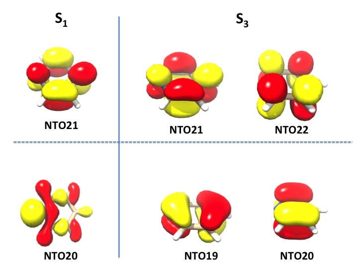
Fig. 7.28 Natural transition orbitals for the pyridine molecule in the S1 and S3 states.
Similar analysis can be performed in the case of ROCIS and DFT/ROCIS calculations as it will be described in section Natural Transition Orbitals/ Natural Difference Orbitals.
7.30.10. Computational Aspects
7.30.10.1. RI Approximation (AO-Basis)
If the SCF calculation used the RI approximation it will also be used in
the TD-DFT calculation. The RI approximation saves a large amount of
time while giving close to identical results (the errors will usually be
\(<\)0.1 eV) and is generally recommended. If the
functional is a hybrid functional the RI-approximation will only be
applied to the Coulomb term while the exchange will be treated as
before. In the SCF you can use this feature with the keyword
(! RIJONX). It will then also be used in the TD-DFT calculation.
Again, the RIJCOSX approximation can be used in TD-DFT and CIS
calculations and leads to very large speedups at virtually no loss in
accuracy.
7.30.10.2. RI Approximation (MO-Basis)
As an alternative to the direct AO-basis computation ORCA allows to use RI-integrals transformed to the MO basis to generate the CI matrix. This algorithm is more disk-intensive. However, for medium sized molecules we have observed speedups on the order of 15 or more with this method. It is particularly benefitial together with hybrid functionals.
In order to use this method you have to specify mode riints in the
%tddft block and you also have to assign an auxiliary basis set (for
example def2-TZVP/C). There is a second algorithm of this kind that is
labelled mode riints_disk
Note that the auxiliary basis set has to be valid for correlation
treatments in case that you have a hybrid functional. Thus the basis
sets developed for RI-MP2 are suitable (def2-SVP/C, def2-TZVP/C and
def2-TZVPP/C). If you have a non-hybrid functional the normal RI-J
auxiliary basis sets are fine.
An example that uses the B3LYP functional is given below:
! RKS B3LYP/G SV(P) def2-SVP/C TightSCF

%tddft
    mode    riints   # or riints_disk (often faster but requires more disk space)
    nroots  8
end

* int 0 1
    C  0 0 0  0.00   0.0   0.0
    O  1 0 0  1.20   0.0   0.0
    H  1 2 0  1.08 120.0   0.0
    H  1 2 3  1.08 120.0 180.0
*
Note
Do not forget to assign a suitable auxiliary basis set! If Hartree-Fock exchange is present (HF or hybrid-DFT) these are the auxiliary bases optimized for correlation while for non-hybrid functionals the standard RI-J bases are suitable.
The standard auxiliary basis sets may not be suitable if you have diffuse functions present and want to study Rydberg states. You have to augment the axuliary basis with diffuse functions yourself in this case.
Be prepared that the transformed integrals take up significant amounts of disk space.
7.30.10.3. Integral Handling
If the SCF calculation is carried out in an integral direct fashion this will also be done in the CIS/TD-DFT calculation. Thus, no bottlenecks arising from large integral transformations or large disk space requirement arise in the calculations. An exception is the MO based RI approximations described in the previous section.
7.30.10.4. Valence versus Rydberg States
For valence excited states the usual orbital basis sets are reasonable. Thus, with polarized double-zeta basis sets sensible results are obtained. Especially DFT calculations have the nice feature of not being overly basis set dependent.
If Rydberg states are desired, you should make sure that diffuse functions are present in your basis set. You could always use the augmented-specific basis, e.g. DEF2-TZVPD, ma-DEF2-TZVP, or aug-cc-pVTZ, or add some extra diffuse basis to your regular basis. These can be added to any “normal” basis set. For example, the following example provides a rather high quality basis for excited state calculations that is based on the Ahlrichs basis set:
%basis
  # augment the carbon basis set by diffuse functions
  addgto 6
    s 1
       1 0.01 1.0
    p 1
       1 0.01 1.0
    d 1
       1 0.07 1.0
    end
end
Tip
If you want to augment a given basis set it is sensible to run a
preliminary SCF calculation and use %output print[p_basis] 2 end.
This will provide you with a detailed listing of basis functions and
their exponents. You can then add additional s, p and perhaps
d-functions with the AddGTO command as in the example above. It is
sensible to decrease the exponent of the diffuse functions by
roughly a factor of 3 from the smallest exponent in the original
basis.
7.30.10.5. Restrictions for Range-Separated Density Functionals
Several restrictions apply for range-separated (hybrid as well as double-hybrid) density functionals. They are currently only implemented to work with the AO-based algorithm within the RIJONX, RIJCOSX, and NORI integral schemes. Additionally, the asymptotic correction has been disabled. However, the nuclear gradient for the excited states is now available, including for the triplets. Please no that the IROOTMULT flag must be set to TRIPLET under %CIS or %TDDFT in order to obtain that.
7.30.10.6. Potential Energy Surface Scans
ORCA allows the combination the scan feature with CIS or TD-DFT. This can be used to map out the excited state potential energy surfaces as a function of one- two- or three parameters. The output of the “trajectory” run automatically contains the excited state energies in addition to the ground state energy. For example consider the following simple job.
! def2-TZVPD
%method scanguess pmodel  # this assignment forces a PModel guess at each step
                          # which is often better if diffuse functions are present
        end
%cis  NRoots        7
      end
%paras rCO = 0.85,1.45,21;
       end
* xyz 0 1
  O  0  0  0
  C  0  0  {rCO}
*
The output file from this job contains the total energies (i.e. the ground state energy plus the excitation energy) for each excited state as a function of C-O bondlength as shown below. Howerver, the assignment of the individual states will change with geometry due to curve crossings. Thus, the state-to-state correlation must be worked out “by hand”. These calculations are nevertheless very helpful in obtaining at least a rough idea about excited state energy surfaces.

Fig. 7.29 Result of a potential energy surface scan for the excited states of
the CO molecule using the orca_cis module.
7.30.10.7. Potential Energy Surface Scans along Normal Coordinates
The ground and excited state potential energy surfaces can also be
mapped as a function of normal coordinates. The normal mode trajectory
run is invoked by the keyword !MTR. In addition several parameters
have to be specified in the block %mtr. The following example
illustrates the use:
First you run a frequency job:
#
! BP86 def2-SV(P) def2/J TightSCF AnFreq

* xyz 0 1
  C       0.000001     -0.000000     -0.671602
  C       0.000000      0.000000      0.671602
  H      -0.000000     -0.940772     -1.252732
  H      -0.000000     -0.940772      1.252732
  H      -0.000000      0.940772     -1.252732
  H      -0.000000      0.940772      1.252732
*
and then:
! BP86 def2-SV(P) def2/J TightSCF MTR

%tddft
  NRoots 3
  triplets false
 end

%mtr
   HessName "ethene.hess"
   modetype normal
   MList 9,13
   RSteps   4,5
   LSteps   4,5
   ddnc     1.0, 0.5
end

* xyz 0 1
  C       0.000001     -0.000000     -0.671602
  C       0.000000      0.000000      0.671602
  H      -0.000000     -0.940772     -1.252732
  H      -0.000000     -0.940772      1.252732
  H      -0.000000      0.940772     -1.252732
  H      -0.000000      0.940772      1.252732
*
The HessName parameter specifies the name of the file which contains
nuclear Hessian matrix calculated in the frequency run. The Hessian
matrix is used to construct normal mode trajectories. The keyword
MList provides the list of the normal modes to be scanned. The
parameters RSteps and LSteps specify the number of steps in positive
and negative direction along each mode in the list. In general, for a
given set of parameters
mlist m1,m2,...mn
rsteps rm1,rm2,...rmn
lsteps lm1,lm2,...lmn
the total number of the displaced geometries for which single point calculations will be performed is equal to \(\prod\limits_{m_{i} } { \left({r_{m_{i} } +l_{m_{i} } +1} \right)}\). Thus, in the present case this number is equal to \(\left({ 4+4+1} \right)\left({ 5+5+1} \right)=99\).
The ddnc parameter specifies increments \(\delta q_{\alpha }\) for
respective normal modes in the list in terms of dimensionless normal
coordinates (DNC’s). The trajectories are constructed so that
corresponding normal coordinates are varied in the range from
\(-l_{\alpha } \delta q_{\alpha }\) to \(r_{\alpha } \delta q_{\alpha }\).
The measure of normal mode displacements in terms DNC’s is appropriate
choice since in spectroscopical applications the potential energy
function \(U\) is usually expressed in terms of the DNC’s. In particular,
in the harmonic approximation \(U(q_{\alpha } )\) has a very simple form
around equilibrium geometry:
where \(\omega_{\alpha }\)is the vibrational frequency of the \(\alpha\)-th mode.
Dimensionless normal coordinate \(q_{\alpha }\) can be related to the vector of atomic Cartesian displacements \(\delta \mathrm{\mathbf{X} }\) as follows:
where \(\left\{{ L_{k\alpha } } \right\}\) is the orthogonal matrix obtained upon numerical diagonalization of the mass-weighted Hessian matrix, and \(\mathrm{\mathbf{M} }\) is the vector of atomic masses. Accordingly, the atomic Cartesian displacements corresponding to a given dimensionless normal coordinate \(q_{\alpha }\) are given by:
Alternatively, it is possible to specify in the input the Cartesian
increment for each normal mode. In such a case, instead of the ddnc
parameter one should use the dxyz keyword followed by the values of
Cartesian displacements, for example:
%mtr
   HessName "ethene.hess"
   modetype normal
   MList 9,13
   RSteps   4,5
   LSteps   4,5
   dxyz     0.01, 0.02 # increments in the Cartesian basis
                       # are given in angstrom units
end
For a given Cartesian increment \(d_{X,\alpha }\) along the \(\alpha\)–th normal mode the atomic displacements are calculated as follows:
The vector \(\mathrm{\mathbf{T} }_{\alpha }\) in the Cartesian basis has components \(T_{i\alpha } =L_{k\alpha } \left({ M_{k} } \right)^{-\frac{1}{2} }\) and length (norm) \(\left\| { \mathrm{\mathbf{T} }_{k} } \right\|\).
The increment length can also be selected on the basis of an estimate
for the expected change in the total energy \(\Delta E\) due to the
displacement according to
eq.(7.118).
The value of \(\Delta E\) can be specified via the EnStep parameter:
%mtr
   HessName "ethene.hess"
   modetype normal
   MList 9,13
   RSteps   4,5
   LSteps   4,5
   EnStep   0.001, 0.001 # the values are given in Eh
end
All quantum chemical methods have to tolerate a certain amount of numerical noise that results from finite convergence tolerances or other cutoffs that are introduced into the theoretical procedures. Hence, it is reasonable to choose \(\Delta E\) such that it is above the characteristic numerical noise level for the given method of calculation.
At the beginning of the program run the following trajectory files which can be visualized in gOpenMol will be created:
BaseName.m9.xyzandBaseName.m13.xyzcontain trajectories along normal modes 9 and 13, respectively.BaseName.m13s1.m9.xyz - BaseName.m13s5.m9.xyzcontain trajectories along normal mode 9 for different fixed displacements along mode 13, so that the fileBaseName.m13sn.m9.xyzcorresponds to the \(n\)-th step in the positive direction along mode 13.BaseName.m13s-1.m9.xyz - BaseName.m13s-5.m9.xyzcontain trajectories along normal mode 9 for different fixed displacements along mode 13, so that the fileBaseName.m13s-n.m9.xyzcorresponds to the \(n\)-th step in the negative direction along mode 13.BaseName.m9s1.m13.xyz - BaseName.m9s4.m13.xyzcontain trajectories along normal mode 13 for different fixed displacements along mode 9, so that the fileBaseName.m9sn.m13.xyzcorresponds to the \(n\)-th step in the positive direction along mode 9.BaseName.m9s-1.m13.xyz - BaseName.m9s-4.m13.xyzcontain trajectories along normal mode 13 for different fixed displacements along mode 9, so that the fileBaseName.m9s-n.m13.xyzcorresponds to the \(n\)-th step in the negative direction along mode 9.
The results of energy single point calculations along the trajectories
will be collected in files BaseName.mtr.escf.S.dat (for the SCF total
energies) and files BaseName.mtr.ecis.S.dat (for the CIS/TDDFT total
energies), where “S” in the suffix of *.S.dat filenames provides
specification of the corresponding trajectory in the same way as it was
done for the case of trajectory files *.xyz (e.g. S=”m9s-1.m13”).
Likewise, the calculated total energies along the trajectories will be
collected in files BaseName.mtr.emp2.S.dat in the case of MP2
calculations, BaseName.mtr.emdci.S.dat (MDCI),
BaseName.mtr.ecasscf.S.dat (CASSCF), BaseName.mtr.emrci.S.dat
(MRCI).
Note, that in principle normal coordinate trajectories can be performed
for an arbitrary number normal modes. This implies that in general
trajectories will contain geometries which involve simultataneous
displacement along several (>2) modes. However, trajectory files
*.xyz and corresponding *.dat files will be generated only for the
structures which are simultaneously displaced along not more than 2
normal coordinates.

Fig. 7.30 Result of a potential energy surface scan along C-C stretching normal
coordinate (mode 13 in the present example) for the excited states of
the ethene molecule using the orca_cis
module.
7.30.10.8. Normal Mode Scan Calculations Between Different Structures
This type of job allows to map PES between two different structures as a
function of normal coordinates. The H\(_{2}\)O molecule represent a
trivial case which has formally 2 equivalent equilibrium structures
which differ by angle H\(_{1}\)—O—H\(_{2}\) ( 103.5\(^{\circ}\) and
256.5\(^{\circ}\), respectively, as follows from the BP86/SV(P)
calculations). In such a case the input for the nomal mode trajectory
run would require the calculation of geometry difference between both
structures in terms of the dimensionless normal coordinates. This can be
done in orca_vib run as follows :
> orca_vib water.hess ddnc geom.xyz
The second parameter ddnc in the command line invokes the calculation of
geometry difference in terms of the DNC’s. Both structures are specified
in the file geom.xyz which has a strict format:
2  3
0
        0.000000      0.000000      0.000000
        0.000000      0.607566      0.770693
        0.000000      0.607566     -0.770693
1
        0.000000      0.000000      0.000000
        0.000000     -0.607566      0.770693
        0.000000     -0.607566     -0.770693
The first line of the input specifies the number of the structures and
total number of atoms (2 and 3, respectively). Specification of each
structure in sequence starts with a new line containing the number of
the structure. The number 0 in the second line is used to denote the
reference structure. Note that atomic coordinates should be given in
units of Å and in the same order as in the ORCA input for the frequency
run from which the file water.hess was calculated.
At the end of the orca_vib run the file geom.ddnc is generated. It
contains the geometry difference in terms of the dimensionless normal
coordinates between the structures with nonzero numbers and the
reference one in geom.xyz :
1
1 9
    0       0.000000
    1       0.000000
    2       0.000000
    3       0.000000
    4       0.000000
    5       0.000000
    6       9.091932
    7      -9.723073
    8       0.000000
The output file indicates that the structural difference occurs along 2 normal coordinates: 6 (bending mode) and 7 (totally symmetric O—H stretching mode). On the basis of the calculated displacement pattern the following input for the normal mode trajectory run between two structures can be designed:
! RKS BP86 SV(P) def2/J  RI TightScf MTR

%mtr
   HessName "water.hess"
   modetype normal
   mlist 6,7
   rsteps   10,0
   lsteps   0, 10
   ddnc     0.9091932, 0.9723073
end

* xyz 0 1
O        0.000000      0.000000      0.000000
H        0.000000      0.607566      0.770693
H        0.000000      0.607566     -0.770693
*
Here the parameters RSteps, LSteps and ddnc are chosen in such a
way that in the scan along modes 6 and 7 the corresponding dimensionless
normal coordinates will be varied in the range 0 \(-\) 9.091932 and
-9.723073 \(-\) 0, respectively, in accordance with the projection pattern
indicated in the file geom.ddnc. Note that normal modes are only
defined up to an arbitrary choice of sign. Consequently, the absolute
sign of the dimensionless displacements is ambiguous and in principle
can vary in different orca_vib runs. It is important that the normal
mode scan between different structures exemplified above is performed
using the same sign of normal modes as in the calculation of normal mode
displacements. This condition is fulfilled if the same normal modes are
used in orca_vib run and trajectory calculation. Thus, since in
orca_vib calculation normal modes are stored in .hess file it is
necessary to use the same Hessian file in the trajectory calculation.
7.30.10.9. Printing Extra Gradients Sequentially
If you want to print extra gradients for external applications or any other reason, you can use the keywords SGRADLIST and TGRADLIST, for singlets and triplets. This will print the gradients sequentially after the CIS/TDDFT run. If you put 0 on the singlet list, the ground state gradient will also be added, always at the end.
%TDDFT SGRADLIST  0, 1, 2
       TGRADLIST  2, 3
END
In order to save this gradients in a text file, please use:
%METHOD STORECISGRAD TRUE END
7.30.11. Keyword List
%cis or %tddft

       NRoots 3            #The number of desired roots
       IRoot  1            #The root to be optimized
       IRootMult Singlet   #or Triplet to optimize it

       MaxDim 5            #Davidson expansion space = MaxDim * NRoots
       MaxIter 35          #Maximum CI Iterations
       NGuessMat 512       #The dimension of the guess matrix
       MaxCore 1024        #The maximum memory to be used on this calculation
       ETol 1e-6           #Energy convergence tolerance
       RTol 1e-6           #Residual Convergence tolerance

       TDA    false        #Switch off for full TDDFT

       LRCPCM true         #Use LRCPCM
       CPCMEQ false        #Which epsilon is used to compute the charges.

       DoNTO               #Generate Natural Transition Orbitals
       NTOStates 1,2,3     #States to consider for NTO analysis. If empty, all will be done.
       NTOThresh 1e-4      #Threshold for printing occupation numbers

       SaveUnrNatOrb       #Saves natural orbitals (not NTO) from unrelaxed densities
                           #for the IROOT chosen (including IROOTLISTs)

       DoSoc     false     #Include spin-orbit coupling?
       SocGrad   false     #Set true to compute the SOC gradient for a given IROOT

       DOTRANS   false     #Transient spectra - starting from IROOT
                 ALL       #Compute all possible transitions