7.19. N-Electron Valence State Pertubation Theory
CASPT2 and NEVPT2 belongs to the family of internally contracted perturbation theories with CASCI reference wavefunctions. Several studies indicate that CASPT2 and NEVPT2 produce energies of similar quality.[366, 757] The NEVPT2 methodology developed by Angeli et al exists in two formulations namely the strongly-contracted NEVPT2 (SC-NEVPT2) and the partially contracted NEVPT2 (PC-NEVPT2). [44, 45, 46] Irrespective of the name “partially contracted” coined by Angeli et al, the latter approach employs a fully internally contracted wavefunction (FIC). Hence, we use the term “FIC-NEVPT2” in place of PC-NEVPT2. ORCA features the fully internally contracted and the strongly contracted NEVPT2. The latter employs strongly contracted CSFs, which form a more compact and orthogonal basis making it computationally slightly more attractive. Hence, the SC-NEVPT2 has been our work horse a for long time. NEVPT2 has many desirable properties - among them:
It is intruder state free due to the choice of the Dyall Hamiltonian [238] as the 0th order Hamiltonian.
The 0th order Hamiltonian is diagonal in the perturber space. Therefore no linear equation system needs to be solved.
It is strictly size consistent. The total energy of two non-interacting systems is equal to the sum of two isolated systems.
It is invariant under unitary transformations within the active subspaces.
“strongly contracted”: Perturber functions only interact via their active part. Different subspaces are orthogonal and hence no time is wasted on orthogonalization issues.
“fully internally contracted”: Invariant to rotations of the inactive and virtual subspaces.
As described in Section
N-Electron Valence State Perturbation Theory (NEVPT2) of the manual, NEVPT2
requires a single keyword on top of a working CASSCF input. The methods
are called within the CASSCF block and detailed settings can be adjusted
in the PTSettings subblock.
We will go through some of the detailed setting in the next few
subsections. For historical reasons, a few features, such as the
quasi-degenerate NEVPT2, are only available for the strongly contracted
NEVPT2. As shown elsewhere, the strong contraction is not a good
starting point for linear scaling
approaches.[806] Thus newer additions such as
the DLPNO and the F12 correction rely on the FIC variant.
[338, 344, 345]
Note that ORCA by default employs
the frozencore approximation, which can be disabled with the simple
keyword !NoFrozenCore. A complete description of the frozecore
settings can be found in section
Frozen Core Options.
%casscf
  ...
  MULT   1,3 # multiplicity block
  NRoots 2,2 # number of roots for the MULT blocks

  CIStep    DMRGCI  # optional to run DMRG-NEVPT2.
                    # default: CSFCI (recommended)
  trafostep ri      # RI approximation for CASSCF and NEVPT2

  # calling the PT2 method of choice
  PTMethod    SC_NEVPT2    # strongly contracted NEVPT2
              FIC_NEVPT2   # fully internally contracted / partially contracted NEVPT2
              DLPNO_NEVPT2 # FIC-NEVPT2 using the DLPNO framework for large molecules

  # detailed settings (optional) for the PT2 approaches
  PTSettings
    NThresh 1e-6     # FIC-NEVPT2 cut off for linear dependencies
    D4Step  Fly      # 4-pdm is constructed on the fly
    D4Tpre  1e-10    # truncation of the 4-pdm
    D3Tpre  1e-14    # trunaction of the 3-pdm
    EWIN  -3,1000    # Energy window for the frozencore setting fc_ewin
    TSMallDenom 1e-2 # printing thresh for small denominators

    # option to skip the PT2 correction for a selected multiplicity block and root
    # (same input structure as weights in %casscf)
    selectedRoots[0]=0,1 # skip the first roots of MULT=1
    selectedRoots[1]=0,0 # skip MULT=3 roots

    # SC-NEVPT2 specific features
    CanonStep 1   # default (exact):canonical orbitals for each state
    QDType    QD_VANVLECK   # QD-SC-NEVPT2: Van Vleck (recommended)

    # FIC-NEVPT2 specific features
    F12       true      # F12-Correction
    Density   unrelaxed # unrelaxed density generated for each state.
    NatOrbs   true      # Computes the natural orbitals

    # DLPNO specific settings
    TCutPNO 1e-8   # controls the accuracy (default 1e-8)

  end

end
NEVPT2 can also be set using the simple keywords on top of any valid CASSCF input.
!SC-NEVPT2       # for the strongly contracted NEVPT2
!FIC-NEVPT2   # for the fully internally contracted NEVPT2
!DLPNO-NEVPT2 # for the DLPNO variant of the FIC-NEVPT2
! ...
%casscf ...
The two computationally most demanding steps of the NEVPT2 calculation are the initial integral transformation involving the two-external labels and the formation of the fourth order density matrix (D4). Efficient approximations to both issues are available in ORCA.
If not otherwise specified (keyword CIStep), CASSCF and consequently
NEVPT2 use a conventional CSF based solver for the CAS-CI problem. In
principle, the NEVPT2 approach can be combined with approximate CI
solution such as the DMRG approach described in section
Density Matrix Renormalization Group. Starting with ORCA 4.0 it is possible to
run NEVPT2-DMRG calculations for the FIC and SC type ansatz using the
methodology developed by the Chan group.[336] Aside
from the usual DMRG input, the program requires an additional parameter
(nevpt2_MaxM) in the DMRG block. However, some of the features will be
restricted to the default CIStep.
%casscf
  cistep DMRGCI
  %dmrg
    ...
    nevpt2_MaxM 2000 # (see Note below)
  end
  PTMethod SC_NEVPT2 # or FIC_NEVPT2
end
For the value nevpt2_MaxM 2000 cf [336].
Using the RI approximation, large molecules with actives spaces of up to
20 orbitals should be computable. The DMRG extension can be combined
with DLPNO and F12 variants. Future version might also support the
CIStep ACCCI and CIStep ICE.
7.19.1. RI, RIJK and RIJCOSX Approximation
Setting the RI approximation on the CASSCF level, will set the RI options for NEVPT2 respectively. The three index integrals are computed and partially stored on disk. Three index integral with two internal labels are kept in main memory. The two-electron integrals are assembled on the fly. The auxiliary basis must be large enough to fit the integrals appearing in the CASSCF orbital gradient/Hessian and the NEVPT2 part. The auxiliary basis set of the type /J does not suffice here.
%casscf
  ...
  TrafoStep RI   # enable RI approximation in CASSCF and NEVPT2
  PTMethod  SC_NEVPT2 # or the NEVPT2 approach or your choice
end
Additional speedups can be obtained if the Fock operator formation is
approximated using the !RIJCOSX or !RIJK techniques. In case of
RIJCOSX, an additional auxiliary basis must be provided for the AuxJ
auxiliary basis slot. For more information on the basis set slots see
section
Built-in Basis Sets.
#RIJCOSX one-liner
! def2-svp def2/J RIJCOSX def2-svp/C

# Commented out: Alternative definition via %basis block
#%basis
#auxJ "def2/J"     # or for example "AutoAux"
#auxC "def2-svp/C" # or for example "AutoAux"
#end
Whereas the RIJK requires a single auxiliary basis set (AuxJK slot),
that is large enough to fit integrals in the Fock-matrix construction,
orbital gradient/Hessian and the correlation part. In contrast to COSX,
the calculation can also be carried out in conv mode (storing the AO
integrals on disk).
#RIJK one-liner, conv is mandatory for RIJK in CASSCF
! def2-svp def2/JK RIJK

# Commented out: Alternative definition via %basis block
#%basis
#auxJK "def2/JK" # or "AutoAux"
#end
The described methodology allows the computation of systems with up to 2000 basis functions. Even larger molecules are accessible in the framework of DLPNO-NEVPT2 described in the next subsection. Several examples can be found in the CASSCF tutorial.
7.19.2. Beyond the RI approximation: DLPNO-NEVPT2
For systems with more than 80 atoms, we recommend the recently developed DLPNO-NEVPT2.[344] It is a successful combination of DLPNO strategy with the FIC-NEVPT2 method. As its single reference counterparts, DLPNO-NEVPT2 recovers 99.9% of the FIC-NEVPT2 correlation energies even for large system. The input structure is similar to the parenting FIC-NEVPT2 method. Below you find an input example for the Fe(II)-complex depicted in Fig. 7.6, where the active space consists of the metal-3d orbitals. The example takes about 9 hour (including 3 hour for one CASSCF iteration) using 8 cores (2.60GHz Intel E5-2670 CPU) for the calculation to finish. A detailed description of the DLPNO-NEVPT2 methodology can be found in our article.[344].
# DLPNO-NEVPT2 calculation for quintet state of FeC72N2H100
!PAL8 def2-TZVP def2/JK
!moread noiter
%moinp "FeC72N2H100.gbw-CASSCF"
%MaxCore 8000
%casscf
  nel 6
  norb 5
  mult 5
  TrafoStep RI # RI approximation is mandatory for DLPNO-NEVPT2

  PTMethod DLPNO_NEVPT2
  # detailed settings (optional)
  PTSettings
    TCutPNO 1e-8   # most important parameter controlling the accuracy (default 1e-8)
    MaxIter   20   # maximum for residual iterations
    MaxDIIS   7    # DIIS dimension
  end
end
*xyz 0 5 FeC72N2H100.xyz
Just like RI-NEVPT2, the calculations requires an auxiliary basis. The aux-basis should be of /C or /JK type (more accurate). Aside from the paper of Guo et al,[344] a concise report of the accuracy can be found in the CASSCF tutorial, where we compute exchange coupling parameters. Note that in the snippet above, we have repeated some of the default setting in the NEVPT sub-block. This is not mandatory and should be avoided to keep the input as simple as possible.
As mentioned earlier, the CASSCF step can be accelerated with the RIJK or RIJCOSX approximation. Both options are equally valid for the DLPNO-NEVPT2. The RIJK variant typically produces more accurate results than RIJCOSX. The input file is almost the same as before, except for the keyword line:
# The combination of RIJK with DLPNO-NEVPT2
!PAL8 def2-TZVP def2/JK conv RIJK
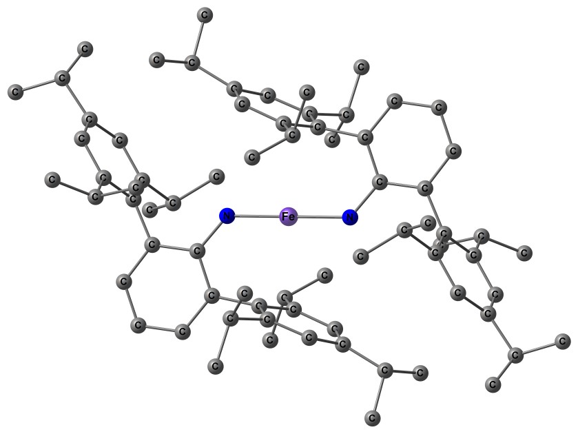
Fig. 7.6 Structure of the FeC\(_{72}\)N\(_{2}\)H\(_{100}\)
7.19.4. Tackling large active CASSCF spaces
Large active spaces (CAS(10,10) and more) require special attention as
the standard implementation involves the fourth order reduced density
matrix (4-RDM).[46] The storage of the latter can easily
reach several gigabytes and thus cannot be kept in core memory. ORCA
thus by default constructs and contracts the 4-RDM on the fly
(D4Step fly). Note that the program can be forced to keep the 4-RDM on
disk (D4Step disk) or in memory (D4Step core).
Aside from the storage, the formation of the 4-RDM itself becomes the
time dominating step of the NEVPT2 calculation for large active spaces.
There are two set of approximations to tackle the challenge. The
prescreening (PS) or the extended prescreening (EPS) approximation and
the cumulant expansion.[343]
In addition, a reformulation of the canonical NEVPT2 is available, that
avoids the 4-RDM.[458] The basic idea of the
latter is similar to the recent development reported by Sokolov and
coworkers.[162] In ORCA the reformulated “efficient”
implementation is combined with the PS approximation. Note that the
reformulation is presently restricted to the canonical NEVPT2 ansatz. An
extension to the DLPNO variant will be available in the future. The new
code is called setting “D4Step efficient”. Irrespective of the
formulation, ORCA by default truncates the CASSCF wave function prior
computation of the fourth order reduced density matrix using the PS
approximation.[342, 343] Only
configurations with a weight larger than a given parameter D4TPre are
taken into account. The same reduction is available for the third order
density matrix using the keyword D3TPre. Both of the parameters can be
adjusted within the PTSettings sub-block of the CASSCF module.
%casscf
  ...
  PTMethod     FIC_NEVPT2  # or SC_NEVPT2

  # detailed settings (optional)
  PTSettings
  D4Step efficient # calling the new NEVPT2 code.
                   # "fly" for the standard code
  D4TPre 1e-12     # default truncation 4-RDM
  D4TPre 1e-14     # default truncation 3-RDM
  imaginary 0.0    # imaginary shift (only for FIC-NEVPT2)
end
These approximations naturally affect the “configuration RI” as well. In this context, it should be noted that a configuration corresponds to a set of configuration state functions (CSF) with identical orbital occupation. For each state the dimension of the CI and and RI space is printed.
D3 Build          ... CI space truncated: 141 -> 82  CFGs
	... RI space truncated: 141 -> 141 CFGs
	D4 Build          ... CI space truncated: 141 -> 82  CFGs
	... RI space truncated: 141 -> 141 CFGs
The default values usually produce errors of less than 1 mEh. However,
the error introduced by the D4TPre is system dependent and should be
double checked. The exact NEVPT2 energy is recovered with the parameters
set to zero. The approximation is available for all variants of NEVPT2
(SC, FIC and DPLNO-FIC). For crude cut-offs, the approximation may lead
to so called false intruder
states.[342, 343, 913]
The behavior shows up as unreasonably large correlation energy
contributions of the 1h (V_i) or 1p (V_a) excitations class e.g.
positive or large correlation energies compared to the 2h-2p (V_ijab)
excitation class. This is a system specific issue, which is avoided with
tighter thresholds (D4TPre=1e-14). The default settings is chosen
conservative and rarely produces artifacts. As last resort, an imaginary
shift can be added to mitigate intruder states. Note that imaginary
shifts (default=0.0 )are restricted the canonical FIC-NEVPT2 - not
DLPNO.
The PS approximation completely neglects CFGs with a small weight. This
is contrasted by the EPS approximation, where the small weights (up to
thresh D4TQuad) are still accounted for (first order
correction).[343]. The results are more robust but
also more expensive compared to the PS approximation.
PTSettings
  D4Step  D4PT  # running the standard code withthe EPS approximation
  D4TPre  1e-12 # default truncation 4-RDM
  D4TQuad 1e-14 # selects CFGs for the first order correction.
end
Huge computational savings can be achieved with the cumulant expansion, which have been recently re-evaluated.[343]. The results should be treated with care as false intruder states can emerge.[913] In these cases, the imaginary level shift is the only mitigation tool. Note that the imaginary shift is implemented only for FIC-NEVPT2.
PTSettings
  D4Step Cu4    # 4-RDM approximated with cumulants
                # "Cu34" to approximate 3-RDM and 4-RDM
  imaginary 0.0 # imaginary shift (only for FIC-NEVPT2)
end
7.19.5. Selecting or Specific States for NEVPT2
ORCA by default computes all states defined in the CASSCF block input
with the NEVPT2 approach. There are cases, where this is not desired and
the user wants to skip some of these states. The input mask of
SelectedRoots is equivalent to the weights keyword in the %casscf
block: The enumeration SelectedRoots[0] refers to the numbering of the
multiplicity blocks and the respective roots defined in CASSCF.
!NEVPT2 ...
%casscf
  ...
  MULT   1,3 # multiplicity block
  NRoots 2,2 # number of roots for the MULT blocks

  # detailed settings (optional) for the PT2 approaches
  PTSettings

    # option to skip the PT2 correction for a selected multiplicity block and root
    # (same input structure as weights in %casscf)
    selectedRoots[0]=0,1 # skip the first roots of MULT=1
    selectedRoots[1]=0,0 # skip MULT=3 roots

  end
end
7.19.6. Unrelaxed Densities and Natural Orbitals
With the FIC-NEVPT2 ansatz, it is possible to request state-specific unrelaxed densities
where \(\Psi_I\) refers to NEVPT2 wave function of the I’th state. The code is implemented using the ORCA AGE tool-chains.[474] In its present form the code runs serial. Note that the density can be used to generate natural orbitals.
%casscf
  ...
  PTMethod     FIC_NEVPT2

  # detailed settings (optional)
  PTSettings
    # densities are disabled by default
    Density Unrelaxed  # unrelaxed density <0+1|E(p,q)|0+1>
            Cu4        # cumulant 4-rdm approximated unrel. density
            Cu34       # cumulant 3/4-rdm approximated unrel. density
            FirstOrder # approximate unrel. density <0|E(p,q)|1>

    NatOrbs True       # off by default
  end
end
The density as well the natural orbitals are state-specific. Thus, ORCA
repeats the population analysis for each state. With the added keyword
!KeepDens the NEVPT2 density is stored in the density container
(.densities file on disk). The latter can be used to create density
plots interactively (see Section
orca_plot). Natural orbitals are stored
in the gbw file-format as .nat file with a prefix corresponding to
the jobname, multiplicity and root. The density can be used to generate
natural orbitals.
A typical output takes the following form:
Unrelaxed Density     ...
Incorizing ADC        ... done in      0.6 sec
Norm <Psi|Psi>        ... done in      0.1 sec (NORM=     1.064186836)
RDM1 <Psi|E|Psi>      ... done in      0.7 sec
Reference Weight      ...     0.939684618
Trace RDM1            ...    20.000000000 (prior correction)

*** Repeating the population analysis with unrelaxed density.
Orbital energies/occupations assumed diagonal. ***
(Note: Temporarily storing unrelaxed densities as cas.scfp)
------------------------------------------------------------------------------
ORCA POPULATION ANALYSIS
------------------------------------------------------------------------------

...
Natural Orbital Occupation Numbers:
...
N[  4] =   1.98812992
N[  5] =   1.98308480
N[  6] =   1.93858508
N[  7] =   1.49303660
N[  8] =   1.49303660
N[  9] =   1.48519842
N[ 10] =   1.48519842
N[ 11] =   0.05922342
N[ 12] =   0.00921465
N[ 13] =   0.00921465
N[ 14] =   0.00794869
N[ 15] =   0.00620254
...
 ===============================================================
 NEVPT2 Results
 ===============================================================
 ...
NEVPT2 natural orbital can be used to do natural orbital iterations
(!MORead NoIter). They might also be a useful tool to find suitable
orbital to extend the active space.[443]
7.19.7. State-averaged NEVPT2
In the definition of the Dyall Hamiltonian [238] the CASSCF orbitals are chosen to diagonalize the Fock operator (pseudo-canonicalized). Therefore, using a state-averaged CASSCF wave function, the NEVPT2 procedure involves the construction and diagonalization of the “state-specific” Fock operators and is thus resulting in a unique set of orbitals for each state. This becomes quickly inefficient for large number of states or large molecular systems since each orbital set implies an integral-transformation. This is the default setting for NEVPT2 and is printed in the output
NEVPT2-SETTINGS:
Orbitals      ... canonical for each state
Other orbital options can be set using the keyword canonstep.
%casscf
  ...
  # detailed settings (optional)
  PTSettings
  canonstep  0 # state-averaged orbitals and specific orbital energies
                 1 # canonical for each state
                 2 # state-averaged orbitals and orbital energies
                 3 # 1-step orbital relaxation
                   # and canonical for each state (partially relaxed)
  end
end
The final orbitals of the state-averaged CASSCF diagonalize the
state-averaged Fock operator. Large computational savings can be made if
these orbitals are employed for all of the states. canonstep 0 chooses
orbital energies as diagonal elements of the state-specific Fock
operators. In release version ORCA 3.0 and older, this has been the
default setting. These options work best if the averaged states are
similar in nature. For SC-NEVPT2, we have implemented two more
canonsteps, which trade accuracy for speed and vice versa.
canonstep 2 is more approximate and employs orbital energies from the
state-averaged calculation. Thus there is no contribution to excitation
energies from the perturber class \(V^{ab}_{ij}\) at this level of
approximation.
If the states under consideration are substantially different, these
approximations will be of poor quality and should be turned off. Better
results can be achieved, if the state-averaged orbitals are partially
relaxed for each state before the actual SC-NEVPT2 calculation.
[224] Often it is not possible to optimize the excited
states separately. Thus canonstep 3 will try a single steepest descent
step for each state before running the actual SC-NEVPT2 calculation with
canonicalized orbitals. Optionally, instead of a steepest descent using
an approximate diagonal Hessian, a single Newton-Raphson step can be
made.
%casscf
  ...
  PTMethod SC_NEVPT2
  # detailed settings (optional)
  PTSettings
  gstep SOSCF true  # steepest descent step
  NR    false       # Newton-Raphson   step
  end
end
Despite a converged state-averaged calculation, the gradient for the individual states can be surprisingly large. As a consequence, the orbital relaxation might fail as both methods might be outside their convergence radius. ORCA will retry the relaxation with an increased damping. If the orbital update still fails, the program will stick with the initial orbitals. Setting an overall damping manually, might help the relaxation procedure.
PTMethod SC_NEVPT2
PTSettings
  gscaling 0.5 # damp gradient with a pre-factor
end
7.19.8. Quasi-Degenerate SC-NEVPT2
NEVPT2 as it is presented in the previous subsections follows the recipe of “diagonalize and perturb”. The 0th order wavefunction is determined by the diagonalization of the CAS-CI matrix. The space spanned by the CAS-CI vectors is often referred to as “model space”. The subsequent perturbation theory is constructed based on the assumption that the states under consideration are well described within the model space. Consequently, the first order correction to the wavefunction \(\Psi^{(1) }_I\) does not affect the composition of the reference state \(\left|I\right\rangle\). Corrections to the wavefunction and energy arise from the interaction of the reference state with the functions \(\left|k\right\rangle\) of the contributing first order interacting space
This is problematic, when the interaction/mixing of states are falsely described at the CASSCF level. A typical example is the dissociation of lithium fluoride.
!def2-tzvp nevpt2 nofrozencore
%casscf
  nel 2
  norb 2 #Li(2s), F(2pz)
  mult 1
  nroots 2
end
%paras
r = 3,7,200
end
*xyz 0 1
Li 0 0 0
F 0 0 {r}
*
Here, the ground and first excited state of \(\Sigma^+\) should not cross. However, at the NEVPT2 level, an erratic double crossing is observed instead.

Fig. 7.7 SC-NEVPT2 and QD-SC-NEVPT2 Li-F dissociation curves of the ground and first excited states for a CAS(2,2) reference
A re-organizing of the reference states can be introduced in the framework of quasi-degenerate perturbation theory. In practice, an effective Hamiltonian is constructed allowing “off-diagonal” corrections to the second order energy
Diagonalization of this eff. Hamiltonian yields improved energies and
rotation matrix (right eigenvectors) that introduces the desired
re-mixing of the reference states. The quasi-degenerate extension to
SC-NEVPT2 [43] can be switched on with the keyword QDType.
%casscf
  ...
  PTMethod SC_NEVPT2     # Must be SC_NEVPT2
  PTSettings
    QDType 0             # disabled (default)
           QD_VanVleck   # Hermitian  eff. Hamiltonian (recommended)
           QD_Bloch      # non-Hermitian eff. Hamiltonian
           QD_Cloiszeaux # Hermitian eff. Hamiltonian

  end
end
ORCA will print the eff. Hamiltonian matrix and its eigenvectors at the end of the calculation.
===============================================================
                      QD-NEVPT2 Results
===============================================================
  *********************
   MULT 1,
  *********************

  Total Hamiltonian to be diagonalized
                  0          1
     0    -107.074594  -0.012574
     1      -0.011748-107.003810

  Right Eigenvectors
                 0          1
    0      -0.987232   0.170171
    1      -0.159292  -0.985414

--------------------------
        ROOT = 0
--------------------------
        Total Energy Correction : dE = -0.25309172934720
        Zero Order Energy       : E0 = -106.82353108218946
        Total Energy (E0+dE)    : E  = -107.07662281153667

--------------------------
        ROOT = 1
--------------------------
        Total Energy Correction : dE = -0.23103459727281
        Zero Order Energy       : E0 = -106.77074682157986
        Total Energy (E0+dE)    : E  = -107.00178141885267
By construction the Hamiltonian is non-Hermitian (QDType QD_Bloch).
Hence the computation of properties with the revised wave function e.g.
expectation values require left- and right eigenvectors. A single set of
eigenvectors (“right”) can be constructed using the Des Cloizeaux scheme
(QDType QD_Cloiszeaux) leading to an Hermitian effective
Hamiltonian.[204] The transformation does not change the
energies but affects the mixing of states. Note that actual eff.
Hamiltonian is printed with a PrintLevel larger 4 in the PTSettings
subblock. The diagonalization of the general matrices appearing in both
formulations may occasionally lead to complex eigenpairs - an undesired
artifact. Although, the eigenvalues have typically only a small
imaginary component, the results are not reliable and ORCA prints a
warning.
--- complex eigenvalues and eigenvectors
  WARNING! QD-Matrix has eigenvalues with imaginary component! iE(0)=-0.000016
  WARNING! QD-Matrix has eigenvalues with imaginary component! iE(1)=0.000016
The QD_VanVleck option avoids the general eigenvalue decomposition.
The equations are derived from second order Van Vleck perturbation
theory, which results in a Hermitian eff. Hamiltonian.[493] The
methodology is equivalent to the symmetrization of the Bloch
Hamiltonian. The solution is always real and properties are easily
accessible. Thus, QD_VanVleck is the recommended approach in ORCA.
For a more detailed comparison of the different eff. Hamiltonian
theories, we refer to the literature.[123, 790]
In all three formulations, the energy denominator in the
quasi-degenerate NEVPT2 is very sensitive to approximations. The
canonicalization options with averaged orbitals and orbitals energies
(canonstep 0/2) have the tendency to lessen the energy-denominator. To
avoid artifacts, the calculation is restricted to canonstep 1 — each
state has its own orbitals.
If properties are requested within the casscf module i.e. zero-field splitting, there will be an additional printing with the “improved” CI vectors and energies. For technical reasons, properties that are not computed in CASSCF such as the Mössbauer parameters do not benefit from the QD-NEVPT2 correction.