6.7. Multireference Configuration Interaction and Pertubation Theory
6.7.1. Introductory Remarks
ORCA contains a multireference correlation module designed for traditional (uncontracted) approaches (configuration interaction, MR-CI, and perturbation theory, MR-PT). For clarification, these approaches have in common that they consider excitations from each and every configuration state function (CSF) of the reference wavefunction. Hence, the computational cost of such approaches grows rapidly with the size of the reference space (e.g. CAS-CI). Internally contracted on the other hand define excitations with respect to the entire reference wavefunction and hence do not share the same bottlenecks. ORCA also features internally contracted approaches (perturbation theory, NEVPT2 and configuration interaction, FIC-MRCI), which are described elsewhere in the manual.
Note
NEVPT2 is typically the method of choice as it is
fast and easy to use. It is highly recommended to check the respective
section, when new to the field. The following chapter focuses on the
traditional multi-reference approaches as part of the orca_mrci
module.
Although there has been quite a bit of experience with it, this part of
the program is still somewhat hard to use and requires patience and
careful testing before the results should be accepted. While we try to
make your life as easy as possible, you have to be aware that ultimately
any meaningful multireference ab initio calculation requires more
insight and planning from the user side than standard SCF or DFT
calculation or single reference correlation approaches like MP2 – so
don’t be fainthearted! You should also be aware that with multireference
methods it is very easy to let a large computer run for a long time and
still to not produce a meaningful result – your insight is a key
ingredient to a successful application! Below a few examples illustrate
some basic uses of the orca_mrci module.
6.7.1.1. RI-approximation
First of all, it is important to understand that the default mode of the
MR-CI module in its present implementation performs a full integral
transformation from the AO to the MO basis. This becomes very laborious
and extremely memory intensive beyond approximately 200 MOs that are
included in the CI. Alternatively, one can construct molecular
electron-electron repulsion integrals from the resolution of the
identity (RI) approximation. Thus a meaningful auxiliary basis set must
be provided if this option is chosen. We recommend the fitting bases
developed by the TurboMole developers for MP2 calculations. These give
accurate transition energies; however, the error in the total energies
is somewhat higher and may be on the order of 1 mEh or so. Check
IntMode to change the default mode for the integral transformation.
Note that in either way, the individually selecting MRCI module requires
to have all integrals in memory which sets a limit on the size of the
molecule that can be studied.
6.7.1.2. Individual Selection
Secondly, it is important to understand that the MR-CI module is of the individually selecting type. Thus, only those excited configuration state functions (CSFs) which interact more strongly than a given threshold (T \(_{\mathbf{sel} })\) with the 0\(^{\text{th} }\) order approximations to the target states will be included in the variational procedure. The effect of the rejected CSFs is estimated using second order perturbation theory. The 0\(^{\text{th} }\) order approximations to the target states are obtained from the diagonalization of the reference space configurations. A further approximation is to reduce the size of this reference space through another selection – all initial references which contribute less than a second threshold (T \(_{\mathbf{pre} })\) to the 0\(^{\text{th} }\) order states are rejected from the reference space.
6.7.1.3. Single excitations
One important aspect concerns the single excitations. If the reference
orbitals come from a CASSCF calculation the matrix elements between the
reference state and the single excitations vanishes and the singles will
not be selected. However, they contribute to fourth and higher orders in
perturbation theory and may be important for obtaining smooth potential
energy surfaces and accurate molecular properties. Hence, the default
mode of the MRCI module requires to include all of the single
excitations via the flag AllSingles =true. This may lead to lengthy
computations if the reference spaces becomes large!
6.7.1.4. Reference Spaces
Third, the reference spaces in the MR-CI module can be of the complete
active space (CAS(n-electrons,m-orbitals) ) or restricted active
space (RAS, explained later) type. It is important to understand
that the program uses the orbitals around the HOMO-LUMO gap as provided
by the user to build up the reference space! Thus, if the orbitals that
you want to put in the active space are not coming “naturally” from your
SCF calculation in the right place you have to reorder them using the
“moread” and “rotate” features together with the NoIter directive.
To select the most meaningful and economic reference space is the most
important step in a multireference calculation. It always requires
insight from the user side and also care and, perhaps, a little trial
and error.
6.7.1.5. Size Consistency
Fourth, it is important to understand that CI type methods are not size consistent. Practically speaking the energy of the supermolecule A-B with noninteracting A and B fragments is not equal to the energies of isolated A and isolated B. There are approximate ways to account for this (ACPF, AQCC and CEPA methods) but the effect will be present in the energies, the more so the more electrons are included in the treatment. The same is not true for the perturbation theory based methods which are size consistent as long as the reference wavefunction is.
6.7.1.6. Performance
There are many flags that control the performance of the MR-CI program. Please refer to chapter 0 for a description of possible flags, thresholds and cut-offs. The most important thresholds are T\(_{\text{sel} }\) and T\(_{\text{pre} }\), and for SORCI also T\(_{\text{nat} }\).

For some methods, like ACPF, it is possible to compare the performance of the MRCI module with the performance of the MDCI module. The MDCI module has been written to provide optimum performance if no approximations are introduced. The MRCI module has ben written more with the idea of flexibility rather than the idea of performance. Let us compare the performance of the two programs in a slightly nontrivial calculation – the zwitter-ionic form of serine. We compare the selecting MRCI approach with the approximation free MDCI module. The molecular size is such that still all four index integrals can be stored in memory.
Module |
Method |
T \(_{\mathbf{sel} }\)(Eh) |
Time (sec) |
Energy (Eh) |
|---|---|---|---|---|
MRCI |
ACPF |
10\(^{-6}\) |
3277 |
-397.943250 |
MDCI |
ACPF |
0 |
1530 |
-397.946429 |
MDCI |
CCSD |
0 |
2995 |
-397.934824 |
MDCI |
CCSD(T) |
0 |
5146 |
-397.974239 |
The selecting ACPF calculation selects about 15% of the possible double excitations and solves a secular problem of size \(\approx\) 360,000 CSFs. The MDCI module ACPF calculation optimizes approximately 2.5 million wavefunction amplitudes — and this is not a large molecule or a large basis set! Despite the fact that the MDCI module makes no approximation, it runs twice as fast as the selected MRCI module and an estimated 50 times faster than the unselected MRCI module! This will become even more pronounced for the larger and more accurate basis sets that one should use in such calculations anyways. The error of the selection is on the order of 3 mEh or 2 kcal/mol in the total energy. One can hope that at least part of this error cancels upon taking energy differences.[1] The more rigorous CCSD calculation takes about a factor of two longer than the ACPF calculation which seems reasonable. The triples add another factor of roughly 2 in this example but this will increase for larger calculations since it has a steeper scaling with the system size. The ACPF energy is intermediate between CCSD and CCSD(T) which is typical — ACPF overshoots the effects of disconnected quadruples which partially compensates for the neglect of triples.
These timings will strongly depend on the system that you run the calculation on. Nevertheless, what you should take from this example are the message that if you can use the MDCI module, do it.
The MDCI module can avoid a full integral transformation for larger systems while the MRCI module can use selection and the RI approximation for larger systems. Both types of calculation will become very expensive very quickly! Approximate MDCI calculations are under development.
6.7.1.7. Symmetry
The MRCI program really takes advantage of symmetry adapted orbitals. In this case the MRCI matrix can be blocked according to irreducible representations and be diagonalized irrep by irrep. This is a big computational advantage and allows one to converge on specific excited states much more readily than if symmetry is not taken into account.
The syntax is relatively easy. If you specify:
newblock 1 *
        nroots 8
        refs cas(4,4) end
        end
Then the “*” indicates that this is to be repeated in each irrep of the point group. Thus, in C\(_{2v}\) the program would calculate 8 singlet roots in each of the four irreps of the C\(_{2v}\) point group thus leading to a total of 32 states.
Alternatively, you can calculate just a few roots in the desired irreps:
newblock 1 0
        nroots 3
        refs cas(4,4) end
        end
      newblock 1 2
        nroots 5
        refs cas(4,4) end
        end
      newblock 3 1
        nroots 1
        refs cas(4,4) end
        end
In this example, we would calculate 3 singlet roots in the irrep “0” (which is A\(_{1})\), then five roots in irrep “2” (which is B\(_{1})\) and then 1 triplet root in irrep 1 (which is B\(_{2})\).
Obviously, the results with and without symmetry will differ slightly. This is due to the fact that without symmetry the reference space will contain references that belong to “wrong” symmetry but will carry with them excited configurations of “right” symmetry. Hence, the calculation without use of symmetry will have more selected CSFs and hence a slightly lower energy. This appears to be unavoidable. However, the effects should not be very large for well designed reference spaces since the additional CSFs do not belong to the first order interacing space.
6.7.2. A Tutorial Type Example of a MR Calculation
Perhaps, the most important use of the MR-CI module is for the calculation of transition energies and optical spectra. Let us first calculate the first excited singlet and triplet state of the formaldehyde molecule using the MR-CI method together with the Davidson correction to approximately account for the effect of unlinked quadruple substitutions. We deliberately choose a somewhat small basis set for this calculation which is already reasonable since we only look at a valence excited state and want to demonstrate the principle.
Suppose that we already know from a ground state calculation that the HOMO of H\(_{2}\)CO is an oxygen lone pair orbitals and the LUMO the \(\pi^{\ast }\) MO. Thus, we want to calculate the singlet and triplet n\(\to \pi ^{\ast }\) transitions and nothing else. Consequently, we only need to correlate two electrons in two orbitals suggesting a CAS(2,2) reference space.
# A simple MRCI example
! def2-SVP def2-SVP/C UseSym

%method frozencore fc_ewin
 		end

%mrci  ewin          -3,1000
       CIType           MRCI
       EUnselOpt     FullMP2
       DavidsonOpt Davidson1
       UseIVOs          true
       tsel             1e-6
       tpre             1e-2
       MaxMemInt         256
       MaxMemVec          32
       IntMode     FullTrafo
       AllSingles       true
       Solver           Diag
       # ground state 1A1
       NewBlock 1 0
         NRoots 1
         Excitations cisd
         Refs CAS(2,2) end
         End
       # HOMO LUMO transition 1A2
       NewBlock 1 1
         NRoots 1
         Excitations cisd
         Refs CAS(2,2) end
         End
       # HOMO LUMO triplet transition 3A2
       NewBlock 3 1
         NRoots 1
         Excitations cisd
         Refs CAS(2,2) end
         end
       end

* int 0 1
 C     0   0   0   0.000000     0.000     0.000
 O     1   0   0   1.200371     0.000     0.000
 H     1   2   0   1.107372   121.941     0.000
 H     1   2   3   1.107372   121.941   180.000
*
This input – which is much more than what is really required - needs
some explanations: First of all, we choose a standard RHF calculation
with the SVP basis set and we assign the SV/C fitting basis although it
is not used in the SCF procedure at all. In the %mrci block all
details of the MR-CI procedure are specified. First, EWin
(%method frozencore fc_ewin) selects the MOs within the given orbital
energy range to be included in the correlation treatment. The CIType
variable selects the type of multireference treatment. Numerous choices
are possible and MRCI is just the one selected for this application.
Note
The CIType statement selects several default values for other variables. So it is a very good idea to place this statement at the beginning of the MR-CI block and possibly overwrite the program selected defaults later. If you place the CIType statement after one of the values which it selects by default your input will simply be overwritten!
The variables EUnselOpt and DavidsonOpt control the corrections to
the MR-CI energies. EUnselOpt specifies the way in which the MR-CI
energies are extrapolated to zero threshold T\(_{\text{Sel} }\). Here we
choose a full MR-MP2 calculation of the missing contributions to be done
after the variational step, i.e. using the relaxed part of the
reference wavefunction as a 0\(^{\text{th} }\) order state for MR-PT. The
DavidsonOpt controls the type of estimate made for the effect of
higher substitutions. Again, multiple choices are possible but the most
commonly used one (despite some real shortcomings) is certainly the
choice Davidson1. The flag UseIVOs instructs the program to use
“improved virtual orbitals”. These are virtual orbitals obtained from a
diagonalization of the Fock operator from which one electron has been
removed in an averaged way from the valence orbitals. Thus, these
orbitals “see” only a \(N-1\) electron potential (as required) and are not
as diffuse as the standard virtual orbitals from Hartree-Fock
calculations. If you input DFT orbitals in the MR-CI moldule (which is
perfectly admittable and also recommended in some cases, for example for
transition metal complexes) then it is recommended to turn that flag off
since the DFT orbitals are already o.k. in this respect. The two
thresholds Tsel and Tpre are already explained above and represent
the selection criteria for the first order interacting space and the
reference space respectively. Tsel is given in units of Eh and refers
to the second order MR-MP2 energy contribution from a given excited CSF.
10\(^{-6}\) Eh is a pretty good value. Reliable results for transition
energies start with \(\approx 10^{-5}\); however, the total energy is
converging pretty slowly with this parameter and this is one of the
greatest drawbacks of individually selecting CI procedures! (see below).
Tpre is dimensionless and refers to the weight of a given initial
reference after diagonalization of the given initial reference space
(10\(^{-4\, }\)is a pretty good value and there is little need to go much
lower. Aggressive values such as 10\(^{-2}\) only select the truly leading
configurations for a given target state which can be time saving.
Intermediate values are not really recommended). The parameters
MaxMemInt and MaxMemVec tell the program how much memory (in MB) it
is allowed to allocate for integrals and for trial and sigma-vectors
respectively.
The flag IntMode tells the program to perform a full integral
transformation. This is possible for small cases with less than, say,
100–200 MOs. In this case that it is possible it speeds up the
calculations considerably. For larger molecules you have to set this
flag to RITrafo which means that integrals are recomputed on the fly
using the RI approximation which is more expensive but the only way to
do the calculation. To switch between the possible modes use:
%mrci  IntMode FullTrafo # exact 4 index transformation
               RITrafo   # use auxiliary basis sets
For small molecules or if high accuracy in the total energies is required it is much better to use the exact four index transformation. The limitations are that you will run out of disk space or main memory with more than ca. 200–300 MOs.
The variable Solver can be diag (for Davidson type diagonalization)
or DIIS for multirrot DIIS type treatments.
%mrci  Solver Diag   # Davidson solver
              DIIS   # Multiroot DIIS
For CI methods, the diag solver is usually preferable. For methods like ACPF that contain nonlinear terms, DIIS is imperative.
Next in the input comes the definition of what CI matrices are to be constructed and diagonalized. Each multiplicity defines a block of the CI matrix which is separately specified. Here we ask for two blocks – singlet and triplet. The general syntax is:
NewBlock Multiplicity Irrep
         NRoots 1           # Number of roots to determine
         Excitations cisd   # Type of excitations
         Refs CAS(NEl,NOrb) end  # Reference space def.
         end                # Finalize the block
Now that all input is understood let us look at the outcome of this calculation:
The first thing that happens after the SCF calculation is the
preparation of the frozen core Fock matrix and the improved virtual
orbitals by the program orca_ciprep. From the output the energies of
the IVOs can be seen. In this case the LUMO comes down to –8.2 eV which
is much more reasonable than the SCF value of \(+\)3….
eV. Concomitantly, the shape of this MO will be much more realistic and
this important since this orbital is in the reference space!
------------------------------------------------------------------------------
                             ORCA CI-PREPARATION
------------------------------------------------------------------------------

Reading the GBW file               ... done
Symmetry usage                     ... ON

One-Electron Matrix                ... test1.H.tmp
GBW-File                           ... test1.gbw
Improved virtual orbitals          ... test1.ivo
First MO in the CI                 ... 2
Internal Fock matrix               ... test1.fi.tmp
LastInternal Orbital               ... 6
Integral package used              ... LIBINT
Reading the GBW file               ... done
Symmetry usage                     ... ON

Reading the one-electron matrix    ... done
Forming inactive density           ... done
Forming averaged valence density   ...
Scaling the occupied orbital occupation numbers
First MO                            ... 2
Last MO                             ... 7
Number of electrons in the range    ...    12
Scaling factor                      ... 0.917

done
Forming internal density           ... done
Forming Fock matrix/matrices       ...
Nuclear repulsion    ...    31.371502
Core repulsion       ...    31.371502
One-electron energy  ...  -114.942080
Fock-energy          ...   -94.993431
Final value          ...   -73.596254
done
Modifying virtual orbitals         ...
Last occupied MO               ...    7
Total number of MOs            ...   38
Number of virtual MOs          ...   30
Doing diagonalization with symmetry
The improved virtual eigenvalues:
    0: -0.2955 au   -8.041 eV    2- B2
    1: -0.0701 au   -1.907 eV    6- A1
    2: -0.0176 au   -0.479 eV    3- B1
    3:  0.0064 au    0.175 eV    7- A1
    4:  0.2922 au    7.951 eV    8- A1
    5:  0.2948 au    8.021 eV    3- B2
    6:  0.3836 au   10.439 eV    4- B1
    7:  0.4333 au   11.790 eV    9- A1
    8:  0.4825 au   13.128 eV    5- B1
    9:  0.5027 au   13.680 eV   10- A1
   10:  0.7218 au   19.642 eV   11- A1
   11:  0.8351 au   22.723 eV    4- B2
   12:  0.9371 au   25.501 eV    6- B1
   13:  1.0265 au   27.933 eV    1- A2
   14:  1.1141 au   30.317 eV   12- A1
   15:  1.2869 au   35.017 eV    5- B2
   16:  1.4605 au   39.743 eV    7- B1
...

done
Transforming integrals             ... done
Storing passive energy             ... done (    -73.59625384 Eh)
Transforming internal FI           ... done
             .... done with the Frozen Core Fock matrices
The next step is to transform the electron-electron repulsion integrals into the MO basis:
-------------------------
SHARK HALF TRANSFORMATION
-------------------------

Number of basis functions                ...     38
Number of operators                      ...      1
   Operator  0:    2-  37

Integral generator used                  ... SHARK
Contraction scheme used                  ... SEGMENTED CONTRACTION
MaxCore in resort                        ...    256 MB

Half transformed integrals for op=   0   ... test1.SHARK_MNPQ0.tmp
Resorted half transformed integrals      ... test1.JAO.tmp
Starting integral generation + half trafo...
Half trafo (segmented) done. Total time =  0.1 sec. integrals=  0.0 sec trafo=  0.0 sec
Starting integral resorting              ... done (  0.0 sec)

SHARK half integral transformation done. Total time =  0.1 sec.


-------------------
FULL TRANSFORMATION
-------------------

Processing MO  10
Processing MO  20
Processing MO  30
Full transformation done
Number of integrals made            ...       222111
Number of integrals stored          ...        59070
Timings:
Time for first half transformation  ...     0.068 sec
Time for second half transformation ...     0.014 sec
Total time                          ...     0.086 sec
This will result in a few additional disk files required by orca_mrci.
The program then tells you which multiplicities will be treated in this
MRCI run:
------------------
CI-BLOCK STRUCTURE
------------------

Number of CI-blocks                ... 3

===========
CI BLOCK 1
===========
Multiplicity             ...   1
Irrep                    ...   0
Number of reference defs ...   1
  Reference   1: CAS(2,2)

Excitation type          ... CISD
Excitation flags for singles:
    1 1 1 1
Excitation flags for doubles:
    1 1 1 / 1 1 1 / 1 1 1

===========
CI BLOCK 2
===========
Multiplicity             ...   1
Irrep                    ...   1
Number of reference defs ...   1
  Reference   1: CAS(2,2)

Excitation type          ... CISD
Excitation flags for singles:
    1 1 1 1
Excitation flags for doubles:
    1 1 1 / 1 1 1 / 1 1 1

===========
CI BLOCK 3
===========
Multiplicity             ...   3
Irrep                    ...   1
Number of reference defs ...   1
  Reference   1: CAS(2,2)

Excitation type          ... CISD
Excitation flags for singles:
    1 1 1 1
Excitation flags for doubles:
    1 1 1 / 1 1 1 / 1 1 1

        --------------------------------------------------------------------
        -------------------- ALL SETUP TASKS ACCOMPLISHED ------------------
        --------------------      (     0.139 sec)        ------------------
        --------------------------------------------------------------------
Now that all the setup tasks have been accomplished the MRCI calculation itself begins.
###################################################
#                                                 #
#                       M R C I                   #
#                                                 #
# TSel    =   1.000e-06 Eh                        #
# TPre    =   1.000e-02                           #
# TIntCut =   1.000e-10 Eh                        #
# Extrapolation to unselected MR-CI by full MP2   #
# DAVIDSON-1 Correction to full CI                #
#                                                 #
###################################################


---------------------
INTEGRAL ORGANIZATION
---------------------

Reading the one-Electron matrix             ... done
E0 read was -73.596253835266
Reading the internal Fock matrix            ... assuming it to be equal to the one-electron matrix!!!
done
Preparing the integral list                 ... done
Loading the full integral                   ... done
Making the simple integrals                 ... done

                  ***************************************
                  *              CI-BLOCK  1            *
                  ***************************************

Configurations with insufficient # of SOMOs WILL be rejected
Building a CAS(2,2) for multiplicity 1 and irrep=A1
Reference Space:
 Initial Number of Configurations :      2
 Internal Orbitals :    2 -    6
 Active Orbitals   :    7 -    8
 External Orbitals :    9 -   37
The number of CSFs in the reference is 2
Calling MRPT_Selection with N(ref)=2
In the first step, the reference space is diagonalized. From this CI,
the most important configurations are selected with Tpre:
------------------
REFERENCE SPACE CI
------------------

 Pre-diagonalization threshold                 : 1.000e-02
Warning: Setting NGuessMat to 512
N(ref-CFG)=2 N(ref-CSF)=2

                       ****Iteration    0****
   Lowest Energy          :  -113.779221580786
   Maximum Energy change  :   113.779221580786 (vector 0)
   Maximum residual norm  :     0.000000000000

      *** CONVERGENCE OF RESIDUAL NORM REACHED ***
Reference space selection using TPre= 1.00e-02

    ... found 1 reference configurations (1 CSFs)
        ... now redoing the reference space CI ...

Warning: Setting NGuessMat to 512
N(ref-CFG)=1 N(ref-CSF)=1

                       ****Iteration    0****
   Lowest Energy          :  -113.778810013503
   Maximum Energy change  :   113.778810013503 (vector 0)
   Maximum residual norm  :     0.000000000000

      *** CONVERGENCE OF RESIDUAL NORM REACHED ***
In this case, the CAS space only has 2 correctly symmetry adapted CSFs one of which (the closed-shell determinant) is selected. In general, larger CAS spaces usually carry around a lot of unnecessary CSFs which are not needed for anything and then the selection is important to reduce the computational effort. The result of the second reference space CI is printed:
----------
CI-RESULTS
----------

The threshold for printing is  0.30 percent
The weights of configurations will be printed. The weights are summed over
all CSFs that belong to a given configuration before printing

STATE   0:  Energy=   -113.778810014 Eh RefWeight=  1.0000  0.00 eV      0.0 cm**-1
      1.0000  : h---h---[20]
Energy is the total energy in Eh. In the present case we can compare
to the SCF energy -113.778810014 Eh and find that the reference space
CI energy is identical, as it has to be since the lowest state coincides
with the reference space. RefWeight gives the weight of the reference
configurations in a CI state. This is 1.0 in the present case since
there were only reference configurations. The number 1.000 is the
weight of the following configuration in the CI vector. The description
of the configuration h—h—[20]p—p— is understood as follows:[2] The
occupation of the active orbitals is explicitly given in square
brackets. Since the HOMO orbitals is number 7 from the SCF procedure,
this refers to MOs 7 and 8 in the present example since we have two
active orbitals. The 2 means doubly occupied, the 0 means empty. Any
number (instead of —) appearing after an h gives the index of an
internal orbital in which a hole is located. Simarly, any number after a
p gives the index of an virtual (external) MO where a particle is
located. Thus h—h—[20] is a closed shell configuration and it
coincides with the SCF configuration—this was of course to be
expected. The second root (in CI-Block 2) h—h—[11] by comparison
refers to the configuration in which one electron has been promoted from
the HOMO to the LUMO and is therefore the desired state that we wanted
to calculate. Things are happy therefore and we can proceed to look at
the output.
The next step is the generation of excited configurations and their
selection based on Tsel:
------------------------------
MR-PT SELECTION TSel= 1.00e-06
------------------------------


Setting reference configurations WITH use of symmetry
Building active patterns WITH use of symmetry

Selection will be done from 1 spatial configurations
Selection will make use of spatial symmetry
 ( 0) Refs        : Sel:         1CFGs/         1CSFs Gen:           1CFGs/           1CSFs  (       0.000 sec)
Building active space densities            ...        0.002 sec
Building active space Fock operators       ...        0.000 sec
 ( 1) (p,q)->(r,s): Sel:         1CFGs/         1CSFs Gen:           1CFGs/           1CSFs  (       0.000 sec)
 ( 2) (i,-)->(p,-): Sel:         1CFGs/         1CSFs Gen:           1CFGs/           1CSFs  (       0.000 sec)
 ( 3) (i,j)->(p,q): Sel:         8CFGs/         8CSFs Gen:           8CFGs/           8CSFs  (       0.000 sec)
 ( 4) (i,p)->(q,r): Sel:         0CFGs/         0CSFs Gen:           1CFGs/           1CSFs  (       0.000 sec)
 ( 5) (p,-)->(a,-): Sel:         8CFGs/         8CSFs Gen:           8CFGs/           8CSFs  (       0.000 sec)
 ( 6) (i,-)->(a,-): Sel:        52CFGs/        52CSFs Gen:          52CFGs/          52CSFs  (       0.000 sec)
 ( 7) (i,j)->(p,a): Sel:        95CFGs/       166CSFs Gen:          96CFGs/         167CSFs  (       0.000 sec)
 ( 8) (i,p)->(q,a): Sel:        21CFGs/        42CSFs Gen:          22CFGs/          44CSFs  (       0.000 sec)
 ( 9) (p,q)->(r,a): Sel:         3CFGs/         3CSFs Gen:           5CFGs/           5CSFs  (       0.000 sec)
 (10) (i,p)->(a,b): Sel:       555CFGs/      1082CSFs Gen:         584CFGs/        1139CSFs  (       0.001 sec)
 (11) (p,q)->(a,b): Sel:       124CFGs/       124CSFs Gen:         148CFGs/         148CSFs  (       0.000 sec)
 (12) (i,j)->(a,b): Sel:      1688CFGs/      2685CSFs Gen:        1887CFGs/        2947CSFs  (       0.001 sec)

Selection results:
Total number of generated configurations:       2814
Number of selected configurations       :       2557 ( 90.9%)
Total number of generated CSFs          :       4522
Number of selected CSFS                 :       4173 ( 92.3%)

The selected tree structure:
Number of selected Internal Portions       :     11
Number of selected Singly External Portions:     27
   average number of VMOs/Portion          :   6.39
   percentage of selected singly externals :  22.83
Number of selected Doubly External Portions:     21
   average number of VMOs/Portion          : 107.59
   percentage of selected doubly externals :  27.76
Here, the program loops through classes of excitations. For each
excitation it produces the excited configurations (CFGs) and from it the
linearly independent spin functions (CSFs) which are possible within the
configuration. It then calculates the interaction with the contracted
\(0^{th}\) order roots and includes all CSFs belonging to a given CFG in
the variational space if the largest second order perturbation energy is
larger or equal to Tsel. In the present case
\(\approx\)136,000 CSFs are produced of which 25% are
selected. For larger molecules and basis sets it is not uncommon to
produce \(10^{9}\)–\(10^{10}\) configurations and then there is no choice
but to select a much smaller fraction than 20%. For your enjoyment, the
program also prints the total energies of each state after selection:
Diagonal second order perturbation results:
State      E(tot)           E(0)+E(1)     E2(sel)      E2(unsel)
             Eh                Eh           Eh           Eh
----------------------------------------------------------------
 0    -114.108350270   -113.778810014    -0.329433    -0.000107
You can ignore this output if you want. In cases that the perturbation
procedure is divergent (not that uncommon!) the total energies look
strange—don’t worry—the following variational calculation is still
OK. The second order perturbation energy is here divided into a selected
part E2(sel) and the part procedure by the unselected configurations
E2(unsel). Depending on the mode of EUnselOpt this value may
already be used later as an estimate of the energetic contribution of
the unselected CSFs.[3]
Now we have \(\approx\) 4,200 CSFs in the variational space of CI block 1 and proceed to diagonalize the Hamiltonian over these CSFs using a Davidson or DIIS type procedure:
------------------------
DAVIDSON-DIAGONALIZATION
------------------------

Dimension of the eigenvalue problem            ...   4173
Number of roots to be determined               ...      1
Maximum size of the expansion space            ...      4
Maximum number of iterations                   ...     35
Convergence tolerance for the residual         ...    1.000e-06
Convergence tolerance for the energies         ...    1.000e-06
Orthogonality tolerance                        ...    1.000e-14
Level Shift                                    ...    0.000e+00
Constructing the preconditioner                ... o.k.
Building the initial guess                     ... o.k.
Number of trial vectors determined             ...      4


                       ****Iteration    0****
   Size of expansion space: 3
   Lowest Energy          :  -113.937028067251
   Maximum Energy change  :   113.937028067251 (vector 0)
   Maximum residual norm  :     0.741727830968

                       ****Iteration    1****
   Size of expansion space: 4
   Lowest Energy          :  -114.082265676116
   Maximum Energy change  :     0.145237608865 (vector 0)
   Maximum residual norm  :     0.012707561344
   Rebuilding the expansion space

                       ****Iteration    2****
   Size of expansion space: 2
   Lowest Energy          :  -114.085350429118
   Maximum Energy change  :     0.003084753001 (vector 0)
   Maximum residual norm  :     0.002880697397

                       ****Iteration    3****
   Size of expansion space: 3
   Lowest Energy          :  -114.086043274125
   Maximum Energy change  :     0.000692845007 (vector 0)
   Maximum residual norm  :     0.000098595378

                       ****Iteration    4****
   Size of expansion space: 4
   Lowest Energy          :  -114.086074300143
   Maximum Energy change  :     0.000031026018 (vector 0)
   Maximum residual norm  :     0.000004959126
   Rebuilding the expansion space

                       ****Iteration    5****
   Size of expansion space: 2
   Lowest Energy          :  -114.086076038587
   Maximum Energy change  :     0.000001738444 (vector 0)
   Maximum residual norm  :     0.000000572348

      *** CONVERGENCE OF RESIDUAL NORM REACHED ***

Storing the converged CI vectors               ... test1.mrci.vec

                 *** DAVIDSON DONE ***
Returned from DIAG section
The procedure converges on all roots simultaneously and finishes after
six iterations which is reasonable. Now the program calculates the
Davidson correction (DavidsonOpt) which is printed for each root.
Davidson type correction:
Root= 0 W=   0.912 E0=  -113.778810014 ECI=  -114.086076039 DE=-0.026913
Already in this small example the correction is pretty large, ca. 27 mEh for the ground state (and \(\approx 36\) mEh for the excited state, later in the output). Thus, a contribution of \(\approx 9\) mEh = 0.25 eV is obtained for the transition energy which is certainly significant. Unfortunately, the correction becomes unreliable as the reference space weight drops or the number of correlated electrons becomes large. Here 0.912 and 0.888 are still OK and the system is small enough to expect good results from the Davidson correction.
The next step is to estimate the correction for the unselected configurations:
Unselected CSF estimate:
Full relaxed MR-MP2 calculation           ...

Selection will be done from 1 spatial configurations
Selection will make use of spatial symmetry
Selection will make use of spatial symmetry
Selection will make use of spatial symmetry
done
Selected MR-MP2 energies                  ...

 Root=  0  E(unsel)=     -0.000106931
In the present case this is below 1 mEh and also very similar for all three states such that it is not important for the transition energy.
----------
CI-RESULTS
----------

The threshold for printing is  0.30 percent
The weights of configurations will be printed. The weights are summed over
all CSFs that belong to a given configuration before printing

STATE   0:  Energy=   -114.113096211 Eh RefWeight=  0.9124  0.00 eV      0.0 cm**-1
      0.9124  : h---h---[20]
      0.0114  : h  6h  6[22]
The final ground state energy is -114.113096211 which is an estimate
of the full CI energy in this basis set. The leading configuration is
still the closed-shell configuration with a weight of \(\approx\) 91%.
However, a double excitation outside the reference space contributes
some 1%. This is the excitation MO6,MO6 \(\to\)LUMO,LUMO. This indicates
that more accurate results are expected once MO6 is also included in the
reference space (this is the HOMO-1). The excited state is dominated by
the HOMO-LUMO transition (as desired) but a few other single- and
double- excitations also show up in the final CI vector.
Now that all CI vectors are known we can order the states according to increasing energy and print (vertical) transition energies:
-------------------
TRANSITION ENERGIES
-------------------

The lowest energy is   -114.113096211 Eh

State Mult Irrep Root Block    mEh          eV      1/cm
  0    1    A1    0    0      0.000      0.000       0.0
  1    3    A2    0    2    134.086      3.649   29428.4
  2    1    A2    0    1    148.499      4.041   32591.8
This result is already pretty good and the transition energies are within \(\approx 0.1\) eV of their experimental gas phase values (\(\approx 3.50\) and \(\approx 4.00\) eV) and may be compared to the CIS values of 3.8 and 4.6 eV which are considerably in error.
In the next step the densities and transition densities are evaluated and the absorption and CD spectra are calculated (in the dipole length formalism) for the spin-allowed transitions together with state dipole moments:
----------------------------------------------------------------------------------------------------
                     ABSORPTION SPECTRUM VIA TRANSITION ELECTRIC DIPOLE MOMENTS
----------------------------------------------------------------------------------------------------
     Transition      Energy     Energy  Wavelength fosc(D2)      D2        DX        DY        DZ
                      (eV)      (cm-1)    (nm)                 (au**2)    (au)      (au)      (au)
----------------------------------------------------------------------------------------------------
  0-1A1 ->  0-1A2   4.040866   32591.8   306.8   0.000000000   0.00000  -0.00000   0.00000   0.00000

------------------------------------------------------------------------------------------
                     CD SPECTRUM VIA TRANSITION ELECTRIC DIPOLE MOMENTS
------------------------------------------------------------------------------------------
     Transition      Energy     Energy  Wavelength    R        MX        MY        MZ
                      (eV)      (cm-1)    (nm)   (1e40*cgs)   (au)      (au)      (au)
------------------------------------------------------------------------------------------
  0-1A1 ->  0-1A2   4.040866   32591.8   306.8   -0.00000  -0.00000  -0.00000   0.59348


------------------------------------------------------------------------------
                             STATE DIPOLE MOMENTS
------------------------------------------------------------------------------
  Root  Block           TX        TY        TZ           |T|
                      (Debye)   (Debye)   (Debye)      (Debye)
------------------------------------------------------------------------------
    0    0            0.00000  -0.00000   2.33244      2.33244
    0    2            0.00000  -0.00000   1.45831      1.45831
    0    1            0.00000  -0.00000   1.58658      1.58658
Here the transition is symmetry forbidden and therefore has no oscillator strength. The state dipole moment for the ground state is 2.33 Debye which is somewhat lower than 2.87 Debye from the SCF calculation. Thus, the effect of correlation is to reduce the polarity consistent with the interpretation that the ionicity of the bonds, which is always overestimated by HF theory, is reduced by the correlation. Finally, you also get a detailed population analysis for each generated state density which may be compared to the corresponding SCF analysis in the preceding part of the output.
This concludes the initial example on the use of the MR-CI module. The
module leaves several files on disk most of which are not yet needed but
in the future will allow more analysis and restart and the like. The
.ivo file is a standard .gbw type file and the orbitals therein can
be used for visualization. This is important in order to figure out the
identity of the generated IVOs. Perhaps they are not the ones you wanted
and then you need to re-run the MR-CI with the IVOs as input, NoIter
and the IVO feature in the new run turned off! We could use the IVOs as
input for a state averaged CASSCF calculation:
! moread UseSym KDIIS
%moinp "Test-SYM-MRCI-H2CO.ivo"

%casscf nel    2
        norb   2
        irrep  0,1,1
        mult   1,1,3
        nroots 1,1,1
        end
If we based a MR-ACPF calculation on this reference space we will find that the calculated transition energies are slightly poorer than in the MRCI+Q calculation. This is typical of approximate cluster methods that usually require somewhat larger reference spaces for accurate results. A similar result is obtained with SORCI.
%mrci  CIType          SORCI
        tsel             1e-6
        tpre             1e-4
        tnat             1e-5
        AllSingles       true
        doNatOrbs        true
        IntMode     FullTrafo
        # ground state 1A1
        NewBlock 1 0
          NRoots 1
          Excitations cisd
          Refs CAS(2,2) end
          End
        # HOMO LUMO transition 1A2
        NewBlock 1 1
          NRoots 1
          Excitations cisd
          Refs CAS(2,2) end
          End
        # HOMO LUMO triplet transition 3A2
        NewBlock 3 1
          NRoots 1
          Excitations cisd
          Refs CAS(2,2) end
          End
end
This gives:
State Mult Irrep Root Block    mEh          eV      1/cm
  0    1    A1    0    0      0.000      0.000       0.0
  1    3    A2    0    2    144.563      3.934   31728.0
  2    1    A2    0    1    161.179      4.386   35374.7
This is systematically 0.4 eV too high. But let us look at the approximate average natural orbital (AANOs) occupation numbers:
------------------------
AVERAGE NATURAL ORBITALS
------------------------

Trace of the density to be diagonalized = 12.000000
Sum of eigenvalues = 12.000000
Natural Orbital Occupation Numbers:
N[  2] ( A1)=   1.99831062
N[  3] ( A1)=   1.99761604
N[  4] ( A1)=   1.99479313
N[  5] ( B1)=   1.99016881
N[  6] ( B2)=   1.95818285
N[  7] ( B1)=   1.33014178
N[  8] ( B2)=   0.70688423
N[  9] ( B1)=   0.00988561
N[ 10] ( A1)=   0.00436843
This shows that there is a low-occupancy orbital (MO6) that has not been part of the reference space. Thus, we try the same calculation again but now with one more active orbital and two more active electrons:
! moread
%moinp "Test-SYM-MRCI-H2CO.gbw"

%casscf nel 4
        norb 3
        irrep  0,1,1
        mult   1,1,3
        nroots 1,1,1
        end

%mrci CIType          SORCI
      tsel             1e-6
      tpre             1e-4
      tnat             1e-5
      AllSingles       true
      doNatOrbs        true
      IntMode     FullTrafo
      # ground state 1A1
      NewBlock 1 0
        NRoots 1
        Excitations cisd
        Refs CAS(4,3) end
        End
      # HOMO LUMO transition 1A2
      NewBlock 1 1
        NRoots 1
        Excitations cisd
        Refs CAS(4,3) end
        End
      # HOMO LUMO triplet transition 3A2
      NewBlock 3 1
        NRoots 1
        Excitations cisd
        Refs CAS(4,3) end
        End
end
This gives:
State Mult Irrep Root Block    mEh          eV      1/cm
  0    1    A1    0    0      0.000      0.000       0.0
  1    3    A2    0    2    145.494      3.959   31932.3
  2    1    A2    0    1    162.222      4.414   35603.6
Which is now fine since all essential physics has been in the reference space. Inspection of the occupation numbers show that there is no suspicious orbital any more. Note that this is still a much more compact calculation that the MRCI+Q.
Likewise, we get an accurate result from MRACPF with the extended reference space.
State Mult Irrep Root Block    mEh          eV      1/cm
  0    1    A1    0    0      0.000      0.000       0.0
  1    3    A2    0    2    134.985      3.673   29625.8
  2    1    A2    0    1    148.330      4.036   32554.6
However, the SORCI calculation is much more compact. For larger molecules the difference becomes more and more pronounced and SORCI or even MRDDCI2 (with or without +Q) maybe the only feasible methods—if at all.
6.7.3. Excitation Energies between Different Multiplicities
As an example for a relatively accurate MRCI+Q calculation consider the following job which calculates the triplet- ground and as the first excited singlet states of O\(_{2}\).
! ano-pVQZ RI-AO cc-pVQZ/JK VeryTightSCF NoPop Conv UseSym RI-MP2 PModel
%mp2 density relaxed natorbs true end
%base "O2"
* xyz 0 3
O  0 0 0
O  0 0 1.2
*

$new_job
! ano-pVQZ RI-AO cc-pVQZ/JK VeryTightSCF NoPop Conv UseSym KDIIS
! moread
%moinp "O2.mp2nat"
%casscf nel     8
        norb    6
        irrep   1,0,1
        nroots  1,2,1
        mult    3,1,1
        trafostep    ri
        switchstep   nr
        end

%mrci   citype mrci
        tsel 1e-7
        tpre 1e-5
        newblock 3 1 nroots 1 refs cas(8,6) end end
        newblock 1 0 nroots 2 refs cas(8,6) end end
        newblock 1 1 nroots 1 refs cas(8,6) end end
        end

* xyz 0 3
O  0 0 0
O  0 0 1.2
*
Note that the linear molecule is run in D\(_{2h}\). This creates a slight problem as the CASSCF procedure necessarily breaks the symmetry of the \(^{1}\Delta\) state.
LOWEST ROOT (ROOT 0, MULT 3, IRREP B1g) =   -149.765383866 Eh -4075.323 eV

STATE   ROOT MULT IRREP DE/a.u.    DE/eV    DE/cm**-1
   1:    0    1  B1g   0.033334     0.907   7316.0
   2:    0    1   Ag   0.033650     0.916   7385.3
   3:    1    1   Ag   0.062381     1.697  13691.1
The result of the MRCI+Q is:
-------------------
TRANSITION ENERGIES
-------------------

The lowest energy is   -150.176905551 Eh

State Mult Irrep Root Block    mEh          eV      1/cm
  0    3   B1g    0    0      0.000      0.000       0.0
  1    1   B1g    0    2     36.971      1.006    8114.2
  2    1    Ag    0    1     38.021      1.035    8344.7
  3    1    Ag    1    1     62.765      1.708   13775.2
These excitation energies are accurate to within a few hundred wavenumbers. Note that the \(\approx 200\) wavenumber splitting in the degenerate \(^{1}\Delta\) state is due to the symmetry breaking of the CAS and the individual selection. Repeating the calculation with the MP2 natural orbitals gives an almost indistinguishable result and a ground state energy that is even lower than what was found with the CASSCF orbitals. Thus, such natural orbitals (that might often be easier to get) are a good substitute for CASSCF orbitals and at the same time the symmetry breaking due to the use of symmetry appears to be difficult to avoid.
-------------------
TRANSITION ENERGIES
-------------------

The lowest energy is   -150.177743426 Eh

State Mult Irrep Root Block    mEh          eV      1/cm
  0    3   B1g    0    0      0.000      0.000       0.0
  1    1   B1g    0    2     37.369      1.017    8201.5
  2    1    Ag    0    1     38.237      1.040    8392.1
  3    1    Ag    1    1     62.731      1.707   13767.9
6.7.4. Correlation Energies
The logic we are following here is the following: CID minus SCF gives the effect of the doubles; going to CISD gives the effect of the singles; QCISD(=CCD) minus CID gives the effect of the disconnected quadruples. QCISD minus QCID gives simultaneously the effect of the singles and the disconnected triples. They are a bit difficult to separate but if one looks at the singles alone and compares with singles + disconnected triples, a fair estimate is probably obtained. Finally, QCISD(T) minus QCISD gives the effect of the connected triples. One could of course also use CCSD instead of QCISD but I felt that the higher powers of T\(_{1}\) obscure the picture a little bit—but this is open to discussion of course.
First H\(_{2}\)O/TZVPP at its MP2/TZVPP equilibrium geometry (\(T_{\text{pre}} \hspace{0.5mm} = \hspace{0.5mm} 10^{-6}\) and \(T_{\text{sel} } \hspace{0.5mm} = \hspace{0.5mm} 10^{-9}\) Eh for the MRCI and MRACPF calculations):
Excitation class |
Energy (Eh) |
Delta-Energy (mEh) |
|---|---|---|
None (RHF) |
-76.0624 |
|
Doubles (CID) |
-76.3174 |
255 |
+Singles (CISD) |
-76.3186 |
1 |
+Disconnected Quadruples (QCID) |
-76.3282 |
11 |
+Disconnected Triples (QCISD) |
-76.3298 |
2 |
+Connected Triples (QCISD(T)) |
-76.3372 |
7 |
CASSCF(8,6) |
-76.1160 |
|
CASSCF(8,6) + MRCI |
-76.3264 |
210 |
CASSCF(8,6) + MRCI+Q |
-76.3359 |
10 |
CASSCF(8,6) + MRACPF |
-76.3341 |
218 |
One observes quite good agreement between single- and multireference approaches. In particular, the contribution of the disconnected triples and singles is very small. The estimate for the disconnected quadruples is fairly good from either the multireference Davidson correction or the ACPF and the agreement between CCSD(T) and these MR methods is 2-3 mEh in the total energy which is roughly within chemical accuracy.
In order to also have an open-shell molecule let us look at NH with a N-H distance of 1.0 Å using the TZVPP basis set.
Excitation class |
Energy (Eh) |
Delta-Energy (mEh) |
|---|---|---|
None (UHF) |
-54.9835 |
|
Doubles (CID) |
-55.1333 |
150 |
+Singles (CISD) |
-55.1344 |
1 |
+Disconnected Quadruples (QCID) |
-55.1366 |
3 |
+Disconnected Triples (QCISD) |
-55.1378 |
1 |
+Connected Triples (QCISD(T)) |
-55.1414 |
4 |
CASSCF(6,5) |
-55.0004 |
|
CASSCF(6,5) + MRCI |
-55.1373 |
137 |
CASSCF(6,5) + MRCI+Q |
-55.1429 |
6 |
CASSCF(6,5) + MRACPF |
-55.1413 |
141 |
Again, the agreement is fairly good and show that both single- and multiple reference approaches converge to the same limit.
6.7.5. Thresholds
Now we choose the CO molecule (1.128 Ångström) with the SVP basis set
and study the convergence of the results with respect to the selection
threshold. Comparison to high level single-reference approaches is
feasible (The SCF energy is -112.645 946 Eh).
6.7.5.1. Reference Values for Total Energies
The single-reference values are:
BD: -112.938 48002
              CCSD: -112.939 79145
             QCISD: -112.941 95700
             BD(T): -112.950 17278
           CCSD(T): -112.950 63889
          QCISD(T): -112.951 37425
         MP4(SDTQ): -112.954 80113
The calculations without connected triples (BD, CCSD, QCISD) are about the best what can be achieved without explicitly considering triple excitations. The CCSD is probably the best in this class. As soon as connected triples are included the CCSD(T), QCISD(T) and BD(T) values are close and from experience they are also close to the full CI values which is then expected somewhere between –112.950 and –112.952 Eh.
6.7.5.2. Convergence of Single Reference Approaches with Respect to T\(_{\text{sel} }\)
Next it is studied how these single reference methods converge with T\(_{\text{sel} }\):
Closed-Shell ACPF:
   Tsel        Energy      (NCSF)    Energy       (NCSF)
   (Eh)       AllSingles=true      AllSingles=false
  TSel=0      -112.943 387 (5671)
  TSel=1e-14  -112.943 387 (2543)  -112.943 387 (2478)
  TSel=1e-10  -112.943 387 (2543)  -112.941 023 (2453)
  TSel=1e-08  -112.943 387 (2451)  -112.937 087 (2346)
  TSel=1e-06  -112.943 350 (2283)  -112.937 046 (2178)
  TSel=1e-05  -112.943 176 (1660)  -112.936 821 (1555)
  TSel=1e-04  -112.944 039 ( 782)  -112.938 381 ( 677)
It is clear that the convergence is erratic if the singles are not automatically included. This is the reason for making this the default from release 2.6.35 on. In the present case singles will only be selected due to round-off errors since by Brillouin’s theorem the singles have zero-interaction with the ground state determinant. Thus, for individually selecting single-reference methods it is a good idea to automatically include all single-excitations in order to get converged results. The alternative would be a different singles selection procedure which has not yet been developed however. The selection of doubles appear to converge the total energies reasonably well. It is seen that the selection selects most CSFs between 10\(^{-5}\) and 10\(^{-7}\) Eh. Already a threshold of 10\(^{-6}\) Eh yields an error of less than 0.1 mEh which is negligible in relation to reaction energies and the like. Even 10\(^{-5}\) Eh gives an error of less than 0.1 kcal/mol.
6.7.5.3. Convergence of Multireference Approaches with Respect to T\(_{\text{pre} }\)
We next turn to multireference treatments. Here we want to correlate all valence electrons in all valence orbitals and therefore a CAS(10,8) is the appropriate choice. We first ask for the converged value of T\(_{\text{pre} }\) by using T\(_{\text{sel} }=\)10\(^{-14}\) and obtain for MRCI\(+\)Q:
TPre = 1e-1: -112.943 964
         1e-2: -112.952 963
         1e-3: -112.953 786
         1e-4: -112.954 019
         1e-5: -112.954 336
         1e-6: -112.954 416
         1e-7: -112.954 440
Thus, pretty good convergence is obtained for T\(_{\text{pre} }=10^{-4}-10^{-6}\). Hence \(10^{-4}\) is the default.
To show a convenient input consider the following:
\
#
# Here we calculate the CO ground state correlation energy with several methods
#
! Def2-SVP Def2-SV/C RI-MP2 CCSD(T)
%base "1"

%mp2  density relaxed
      donatorbs  true
      end

* int 0 1
 C     0   0   0   0.000000     0.000     0.000
 O     1   0   0   1.128        0.000     0.000
*

$new_job

! aug-SVP MRACPF
! moread
%moinp "1.mp2nat"
# the CASSCF is done with MP2 natural orbitals which is a good idea and
# secondly we use a large level shift in order to help convergence
%casscf nel     10
        norb     8
        mult     1
        nroots   1
        shiftup  2
        shiftdn  2
        end

%mrci   tsel 1e-8
        tpre 1e-6
        end

* int 0 1
 C     0   0   0   0.000  0.000  0.000
 O     1   0   0   1.128  0.000  0.000
*
This job computes at the same time all of the below and demonstrates once more the agreement between consequent single- and multireference correlation methods
SCF          =  -112.6459
RI-MP2       =  -112.9330
CCSD         =  -112.9398
CCSD(T)      =  -112.9506
CASSCF(10,8) =  -112.7769
MRACPF       =  -112.9514
6.7.6. Energy Differences - Bond Breaking
For the calculation of energy differences we start again with the reference CCSD(T) calculation; this method is one of the few which can claim chemical accuracy in practical applications:
Reference Total Energies for N2 at 1.0977 Angstr\"{o}m with
  The SVP basis
    E(CCSD)   = -109.163 497
    E(CCSD(T))= -109.175 625
  Nitrogen Atom (4S), SVP basis, unrestricted
    E(CCSD)   =  -54.421 004
    E(CCSD(T))=  -54.421 7183
  Energy Difference:
  Delta-E(CCSD)   = -0.321 489 = 8.75 eV
  Delta-E(CCSD(T))= -0.332 188 = 9.04 eV
The basis set is of course not suitable for quantitative comparison to experimental values. However, this is not the point here in these calculations which are illustrative in nature. The SVP basis is just good enough to allow for a method assessment without leading to excessively expensive calculations.
This is now to be compared with the corresponding energy differences computed with some single-reference approaches. A typical input is (this is a somewhat old-fashioned example – in the present program version you would do a full valence CASSCF(10,8) or CASSCF(6,6) and invoke the MR-methods with a single keyword):
! HF def2-SVP def2-TZVPP/C VeryTightSCF NoPop

%base "1"

* xyz 0 1
N 0 0 0
N 0 0 1.0977
*
%method
     frozencore fc_ewin
end

%mrci
     EWin          -3,1000
     CIType       MRACPF2a
     Solver           DIIS
     IntMode      FullTrafo
     UseIVOs          true
     AllSingles       true
     TSel            1e-14
     TPre            1e-05
     TNat              0.0
     ETol            1e-10
     RTol            1e-10
     NewBlock 1 *
          NRoots 1
          Excitations CISD
          refs CAS(0,0) end
     end
end

$new_job

! ROHF def2-SVP def2-TZVPP/C VeryTightSCF NoPop PModel

%base "2"

* xyz 0 4
N 0 0 0
*
%method
       frozencore fc_ewin
end

%mrci
      EWin          -3,1000
      CIType       MRACPF2a
      IntMode      FullTrafo
      UseIVOs          true
      AllSingles       true
      TSel            1e-14
      TPre            1e-05
      TNat              0.0
      ETol            1e-10
      RTol            1e-10
      NewBlock 4 *
          NRoots 1
          Excitations CISD
          refs CAS(3,3) end
      end
end
The results are:
Single reference approaches:
  Method   N2-Molecule         N-Atom        Delta-E
  CISD+Q : -109.167 904        -54.422 769    8.77 eV
  ACPF   : -109.166 926        -54.421 783    8.80 eV
  ACPF2  : -109.166 751        -54.421 333    8.82 eV
  ACPF2a : -109.166 730        -54.421 186    8.83 eV
  CEPA1  : -109.159 721        -54.422 564    8.56 eV
  CEPA2  : -109.172 888        -54.422 732    8.91 eV
  CEPA3  : -109.161 034        -54.422 589    8.59 eV
  AQCC   : -109.160 574        -54.420 948    8.67 eV
  CEPA-0 : -109.174 924        -54.422 951    8.95 eV
With exception is CEPA1 and CEPA3, the results are OK. The reason for the poor performance of these methods is simply that the formalism implemented is only correct for closed shells – open shells require a different formalism which we do not have available in the MRCI module (but in the single reference MDCI module). Due to the simple approximations made in CEPA2 it should also be valid for open shells and the numerical results are in support of that.
Next we turn to the multireference methods and take a CAS(10,8) reference as for CO in order to correlate all valence electrons. [4]
Multi reference approaches:
  Method     N2-Molecule         N-Atom        Delta-E
  MRCISD+Q: -109.180 089        -54.422 667    9.11 eV
  MRACPF  : -109.178 708        -54.421 685    9.12 eV
  MRACPF2 : -109.177 140        -54.421 236    9.11 eV
  MRAQCC  : -109.175 947        -54.420 851    9.10 eV
  SORCI   : -109.179 101        -54.422 703    9.08 eV
This test calculation pleasingly shows the high consistency of multireference approaches which all converge more or less to the same result which must be accurate.
6.7.7. Energy Differences - Spin Flipping
There are a number of interesting situations in which one is interested in a small energy difference which arises from two states of different multiplicity but same orbital configuration. This is the phenomenon met in diradicals or in magnetic coupling in transition metal complexes. As a primitive model for such cases one may consider the hypothetical molecule H-Ne-H in a linear configuration which will be used as a model in this section.
The reference value is obtained by a MR-ACPF calculation with all valence electrons active (again, this example is somewhat old fashioned – in the present program version you would do a CASSCF calculation followed by MR methods with a single keyword):
! ROHF def2-SVP def2-TZVPP/C VeryTightSCF NoPop
%basis
     NewAuxCGTO Ne "AutoAux" end
end
* xyz 0 3
H  0 0 0
Ne 0 0 2.0
H  0 0 4.0
*
%method frozencore fc_ewin
        end

%mrci  EWin       -3,1000
       CIType     MRACPF2a
       IntMode   FullTrafo
       Solver         DIIS
       UseIVOs        true
       TSel              0
       TPre          1e-10
       ETol          1e-09
       RTol          1e-09
       DoDDCIMP2      true
       NewBlock 1 *
          NRoots 1
          Excitations CISD
          refs CAS(10,6) end
          end
       NewBlock 3 *
          NRoots 1
          Excitations CISD
          refs CAS(10,6) end
          end
       end
which gives the reference value 108 cm\(^{-1}\). We now compare that to several other methods which only have the two “magnetic” orbitals (the 1s’s on the hydrogens) in the active space:
... same as above
%mrci  EWin       -10,1000
       CIType      MRDDCI3
       ... same as previously
       NewBlock 1 *
          NRoots 1
          refs CAS(2,2) end
          end
       NewBlock 3 *
          NRoots 1
          refs CAS(2,2) end
          end
       end
This gives the result:
Method      S-T gap
MR-CI+Q  :  98 cm-1
MR-CI    :  93 cm-1
MR-ACPF  :  98 cm-1
MR-ACPF2 :  98 cm-1
MR-ACPF2a:  97 cm-1
MR-AQCC  :  95 cm-1
SORCI    : 131 cm-1
MR-DDCI2 :  85 cm-1
MR-DDCI3 : 130 cm-1
All these methods give good results with SORCI leading to a somewhat larger error than the others. The (difference dedicated CI) DDCI2 method slightly underestimates the coupling which is characteristic of this method. It is nice in a way that DDCI3 gives the same result as SORCI since SORCI is supposed to approximate the DDCI3 (or better the IDDCI3) result which it obviously does.
This splitting can also be studied using broken symmetry HF and DFT methods as explained elsewhere in this manual:
Method    S-T gap
 UHF     : 70 cm-1
 B3LYP/G : 240 cm-1
 BP86    : 354 cm-1
 PW91    : 234 cm-1
 PBE     : 234 cm-1
 PBE0    : 162 cm-1
 RPBE    : 242 cm-1
This confirms the usual notions; UHF underestimates the coupling and DFT overestimates it, less so for hybrid functionals than for GGAs. The BP86 is worse than PW91 or PBE. The PBE0 hybrid may be the best of the DFT methods. For some reason most of the DFT methods give the best results if the BS state is simply taken as an approximation for the true open-shell singlet. This is, in our opinion, not backed up by theory but has been observed by other authors too.
Now let us study the dependence on T\(_{\text{sel} }\) as this is supposed to be critical (we use the DDCI3 method):
Tsel     S-T gap
    1e-04     121
    1e-05     128
    1e-06     132
    1e-07     131
    1e-08     131
    1e-10     131
    1e-12     131
    0         131
The convergence is excellent once AllSingles are included.
6.7.8. Potential Energy Surfaces
Another situation where multireference approaches are necessary is when bond breaking is studied and one wants to calculate a full potential energy surface. Say we want to compute the potential energy surface of the CH molecule. First we have to figure out which states to include. Hence, let us first determine a significant number of roots for the full valence CASSCF reference state (we use a small basis set in order to make the job fast).
! ANO-pVDZ VeryTightSCF NoPop Conv

%casscf nel      5
        norb     5
        nroots   2
        mult     2
        end

%mrci  CIType      MRCI
       NewBlock 2 *
         excitations none
         NRoots 15
         refs CAS(5,5) end
         end
       NewBlock 4 *
         excitations none
         NRoots 15
         refs CAS(5,5) end
         end
       end

* xyz 0 2
C  0 0 0
H  0 0 1.15
*
This yields:
-------------------
TRANSITION ENERGIES
-------------------

The lowest energy is    -38.308119994 Eh

State Mult Irrep Root Block    mEh          eV      1/cm
  0    2    -1    0    0      0.000      0.000       0.0
  1    2    -1    1    0      0.000      0.000       0.0
  2    4    -1    0    1     14.679      0.399    3221.6
  3    2    -1    2    0    126.464      3.441   27755.7
  4    2    -1    3    0    126.464      3.441   27755.7
  5    2    -1    4    0    132.689      3.611   29121.8
  6    2    -1    5    0    164.261      4.470   36051.2
  7    2    -1    6    0    305.087      8.302   66958.9
  8    2    -1    7    0    305.087      8.302   66958.9
  9    4    -1    1    1    328.911      8.950   72187.7
 10    4    -1    2    1    452.676     12.318   99350.8
 11    4    -1    3    1    452.676     12.318   99350.8
 12    2    -1    8    0    460.116     12.520  100983.9
 13    2    -1    9    0    463.438     12.611  101712.9
 14    2    -1   10    0    463.438     12.611  101712.9
 ...
Thus, if we want to focus on the low-lying states we should include five doublet and one quartet root. Now we run a second job with these roots and scan the internuclear distance.
! ano-pVDZ VeryTightSCF NoPop Conv MRCI+Q

%casscf nel     5
        norb    5
        nroots  5,1
        mult    2,4
        shiftup 2
        end

%paras R = 0.8,2.5,25
       end

* xyz 0 2
C  0 0 0
H  0 0 {R}
*
The surfaces obtained in this run are shown in
Fig. 6.30. You can nicely
see the crossing of the \(^{2}\Sigma\) and \(^{2}\Delta\) states fairly
close to the equilibrium distance and also the merging of the
\(^{4}\Sigma\) state with \(^{2}\Pi\) and \(^{2}\Sigma\) towards the asymptote
that where C-H dissociates in a neutral C-atom in its \(^{3}\)P ground
state and a neutral hydrogen atom in its \(^{2}\)S ground state. You can
observe that once AllSingles is set to true (the default), the default
settings of the MRCI module yield fairly smooth potential energy
surfaces.

Fig. 6.30 Potential energy surfaces for some low-lying states of CH using the MRCI+Q method
In many cases one will focus on the region around the minimum where the surface is nearly quadratic. In this case one can still perform a few (2, 3, 5, ) point polynomial fitting from which the important parameters can be determined. The numerical accuracy and the behavior with respect to \(T_\text{sel}\) has to be studied in these cases since the selection produces some noise in the procedure. We illustrate this with a calculation on the HF molecule:
! ano-pVDZ VeryTightSCF NoPop Conv MRCI+Q

%paras  R = 0.85,1.1,7
        end

%casscf nel     8
        norb    5
        nroots  1  mult    1
        shiftup 2.5 shiftdn 2.5 switchstep nr gtol    1e-5
        end

%mrci   tsel 1e-8
        tpre 1e-5
        end

* xyz 0 1
F  0 0 0
H  0 0 {R}
*
The output contains the result of a Morse fit:
Morse-Fit Results:
 Re               =   0.93014 Angstroem
 we               =   4111.2 cm**-1
 wexe             =     79.5 cm**-1
Which may be compared with the CCSD(T) values calculated with the same basis set:
Morse-Fit Results:
 Re               =   0.92246 Angstroem
 we               =   4209.8 cm**-1
 wexe             =     97.6 cm**-1
The agreement between MRCI+Q and CCSD(T) results is fairly good.
6.7.9. Multireference Systems - Ozone
The ozone molecule is a rather classical multireference system due to its diradical character. Let us look at the three highest occupied and lowest unoccupied MO (the next occupied MO is some 6 eV lower in energy and the next virtual MO some 10 eV higher in energy):
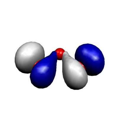 (a) MO-9
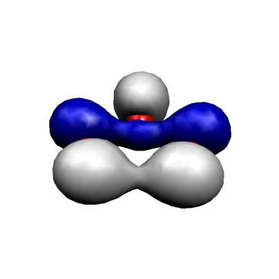 (b) MO-10
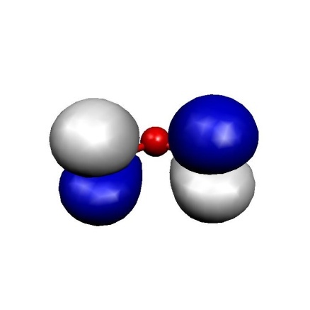 (c) MO 11(HOMO)
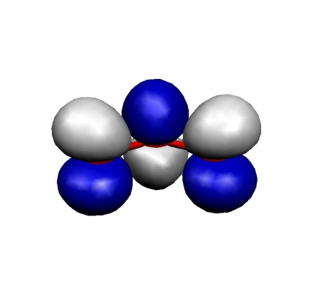 (d) MO 12(LUMO)
Fig. 6.31 Frontier MOs of the Ozone Molecule.
These MOs are two \(\sigma\) lone pairs which are high in energy and then the symmetric and antisymmetric combinations of the oxygen \(\pi\) lone pairs. In particular, the LUMO is low lying and will lead to strong correlation effects since the (HOMO)\(^{2} \to \) (LUMO)\(^{2}\) excitation will show up with a large coefficient. Physically speaking this is testimony of the large diradical character of this molecule which is roughly represented by the structure \(\uparrow\)O-O-O\(\downarrow\). Thus, the minimal active space to treat this molecule correctly is a CAS(2,2) space which includes the HOMO and the LUMO. We illustrate the calculation by looking at the RHF, MP2 MRACPF calculations of the two-dimensional potential energy surface along the O–O bond distance and the O-O-O angle (experimental values are 1.2717 Å and 116.78\({^\circ}\)).
! ano-pVDZ VeryTightSCF NoPop MRCI+Q Conv

%paras R     = 1.20,1.40,21
       Theta = 100,150,21
       end

%casscf nel     2
        norb    2
        mult    1
        nroots  1
        end

%mrci   tsel    1e-8
        tpre    1e-5
        end

* int 0 1
O  0 0 0  0   0         0
O  1 0 0 {R}  0         0
O  1 2 0 {R}  {Theta}   0
*
This is a slightly lengthy calculation due to the 441 energy evaluations required. RHF does not find any meaningful minimum within the range of examined geometries. MP2 is much better and comes close to the desired minimum but underestimates the O–O distance by some 0.03 Å. CCSD(T) gives a very good angle but a O–O distance that is too long. In fact, the largest doubles amplitude is \(\approx\) 0.2 in these calculations (the HOMO–LUMO double excitation) which indicates a near degeneracy calculation that even CCSD(T) has problems to deal with. Already the CAS(2,2) calculation is in qualitative agreement with experiment and the MRCI\(+\)Q calculation then gives almost perfect agreement.
The difference between the CCSD(T) and MRCI\(+\)Q surfaces shows that the CCSD(T) is a bit lower than the MRCI\(+\)Q one suggesting that it treats more correlation. However, CCSD(T) does it in an unbalanced way. The MRCI calculation employs single and double excitations on top of the HOMO-LUMO double excitation, which results in triples and quadruples that apparently play an important role in balancing the MR calculation. These excitations are treated to all orders explicitly in the MRCI calculation but only approximately (quadruples as simultaneous pair excitations and triples perturbatively) in the coupled-cluster approach. Thus, despite the considerable robustness of CC theory in electronically difficult situations it is not applicable to genuine multireference problems.
This is a nice result despite the too small basis set used and shows how important it can be to go to a multireference treatment with a physically reasonable active space (even if is only \(2 \times 2\)) in order to get qualitatively and quantitatively correct results.
 (a) RHF
 (b) CASSCF(2,2)
 (c) MP2
 (d) CCSD(T)
 (e) MRCI+Q
 (f) Difference CCSD(T)/MRCI+Q
Fig. 6.32 2D potential energy surface for the \( O_3 \) molecule calculated with different methods
6.7.10. Size Consistency
Finally, we want to study the size consistency errors of the methods. For this we study two non-interacting HF molecules at the single reference level and compare to the energy of a single HF molecule. This should give a reasonably fair idea of the typical performance of each method (energies in Eh)[5]:
E(HF)         E(HF+HF)  |Difference|
  CISD+Q   -100.138 475  -200.273 599     0.00335
  ACPF     -100.137 050  -200.274 010     0.00000
  ACPF2    -100.136 913  -200.273 823     0.00000
  AQCC     -100.135 059  -200.269 792     0.00032
The results are roughly as expected – CISD+Q has a relatively large error, ACPF and ACPF/2 are perfect for this type of example; AQCC is not expected to be size consistent and is (only) about a factor of 10 better than CISD+Q in this respect. CEPA-0 is also size consistent.
6.7.11. Efficient MR-MP2 Calculations for Larger Molecules
Uncontracted MR-MP2 approaches are nowadays outdated. They are much more expensive than internally contracted e.g. the NEVPT2 method described in section N-Electron Valence State Pertubation Theory. Moreover, MR-MP2 is prone to intruder states, which is a major obstacle for practical applications. For historical reasons, this section is dedicated to the traditional MR-MP2 approach that is available since version 2.7.0 ORCA. The implementation avoids the full integral transformation for MR-MP2 which leads to significant savings in terms of time and memory. Thus, relatively large RI-MR-MP2 calculations can be done with fairly high efficiency. However, the program still uses an uncontracted first order wavefunction which means that for very large reference space, the calculations still become untractable.
Consider for example the rotation of the stilbene molecule around the central double bond
 (a)
(a)
 (b)
(b)
Fig. 6.33 Rotation of stilbene around the central double bond using a CASSCF(2,2) reference and correlating the reference with MR-MP2.
The input for this calculation is shown below. The calculation has more than 500 basis functions and still runs through in less than one hour per step (CASSCF-MR-MP2). The program takes care of the reduced number of two-electron integrals relative to the parent MRCI method and hence can be applied to larger molecules as well. Note that we have taken a “JK” fitting basis in order to fit the Coulomb and the dynamic correlation contributions both with sufficient accuracy. Thus, this example demonstrates that MR-MP2 calculations for not too large reference spaces can be done efficiently with ORCA (as a minor detail note that the calculations were started at a dihedral angle of 90 degrees in order to make sure that the correct two orbitals are in the active space, namely the central carbon p-orbitals that would make up the pi-bond in the coplanar structure).
#
# Stilbene rotation using MRMP2
#
! def2-TZVP def2/JK RIJCOSX RI-MRMP2

%casscf nel            2
        norb           2
        end

%mrci   maxmemint 2000
        tsel 1e-8
        end


%paras  DIHED = 90,270, 19
        end

* int 0 1
 C     0   0   0   0.000000     0.000     0.000
 C     1   0   0   1.343827     0.000     0.000
 C     2   1   0   1.490606   125.126     0.000
 C     1   2   3   1.489535   125.829   \{DIHED\}
 C     4   1   2   1.400473   118.696   180.000
 C     4   1   2   1.400488   122.999     0.000
 C     6   4   1   1.395945   120.752   180.000
 C     5   4   1   1.394580   121.061   180.000
 C     8   5   4   1.392286   120.004     0.000
 C     3   2   1   1.400587   118.959   180.000
 C     3   2   1   1.401106   122.779     0.000
 C    11   3   2   1.395422   120.840   180.001
 C    12  11   3   1.392546   120.181     0.000
 C    13  12  11   1.392464   119.663     0.000
 H     1   2   3   1.099419   118.266     0.000
 H     2   1   3   1.100264   118.477   179.999
 H     5   4   1   1.102119   119.965     0.000
 H     6   4   1   1.100393   121.065     0.000
 H     7   6   4   1.102835   119.956   180.000
 H     8   5   4   1.102774   119.989   180.000
 H     9   8   5   1.102847   120.145   180.000
 H    10   3   2   1.102271   120.003     0.000
 H    11   3   2   1.100185   121.130     0.000
 H    12  11   3   1.103001   119.889   180.000
 H    13  12  11   1.102704   120.113   180.000
 H    14  13  12   1.102746   119.941   180.000
*
6.7.12. Keywords
Here is a reasonably complete list of Keywords and their meaning. Note that the MRCI pogram is considered legacy and we can neither guarantuee that the keywords still work as intended, nor is it likely that somebody will be willing or able to fix a problem with any of them. Additional information is found in section 9.
%mrci
  CIType	MRCI
  		MRDDCI1
      		MRDDCI2
      		MRDDCI3
		SORCI
 		SORCP
		MRACPF
 		MRACPF2
		MRACPF2a
		MRAQCC
		MRCEPA_R
		MRCEPA_0
		MRMP2
 		MRMP3
		MRRE2
		MRRE3
		MRRE4
		CEPA1
		CEPA2
		CEPA3

      # CSF selection and convergence thresholds
      TSel            1e-14    # selection threshold
      TPre            1e-05    # pre-diagonalization threshold
      TNat              0.0      #
      ETol            1e-10
      RTol            1e-10

      # Size consistency corrections and the like
      EUnselOpt    MaxOverlap
                           FullMP2
      DavidsonOpt Davidson1
                           Davidson2
                           Siegbahn
                           Pople
        NELCORR   15   # number of electrons correlated for MRACPF and
        the like


      # MRPT stuff
      UsePartialTrafo   true/false    # speedups MRMP2
      UseDiagonalContraction true/false # legacy
      Partitioning  EN    # Epstein Nesbet
                          MP    # Moeller Plesset
                          RE     # Fink's partitioning
       FOpt           Standard   # choice of Fock operators to be
       used in MRPT
                         G0
                         G3
       H0Opt        Diagonal
                         Projected
                         Full
     MRPT_b            0.2   # intruder state fudge factor
     MRPT_SHIFT     1.0   # level shift

       # Integral handling
       IntMode     FullTrafo   # exact transformation (lots of memory)
                         RITRafo     # RI integrals (slow!)
      UseIVOs      true/false  # use improved virtual orbitals?

      # Try at your own risk
      CIMode    Auto
                     Conv
                     Semidirect
                     Direct
                     Direct2
                     Direct3

      # orbital selection
      EWin          epsilon_min,epsilon_max   # orbital energy window
      MORanges  First_internal, Last_Internal, First_active,
      Last_Active, First-Virtual,Last_virtual  # alternative MO
      definition
      XASMOs  x1,x2,x3,...   # List of XAS donor MOs (see above)

      #density generation
     Densities StateDens, TransitionDens
         # StateDens= GS, GS_EL, GS_EL_SPIN, ALL_LOWEST,
         ALL_LOWEST_EL, ALL_LOWEST_EL_SPIN, ALL, ALL_EL, ALL_EL_SPIN
        # TransitionDens= FROM_GS_EL, FROMGS_EL_SPIN,FROM_LOWEST_EL, \\ FROM_LOWEST_EL_SPIN,FROM_ALL_EL,FROM_ALL_EL_SPIN
      # Memory
     MaxMemVec  1024 # in MB
     MaxMemInt   1024 #  in MB


    # Diagonalizer
    Solver DIIS
              DIAG
              NEWDVD
     MaxDIIS
     RelaxRefs true/false
     LevelShift 0.0
     MaxDim  15
     NGuessMat 10
     MaxIter 25
     NGuessMatRefCI  100
     DVDShift  1.0


      # Bells and whistles
      KeepFiles    true/false
      AllSingles       true/false    # Force all singles to be included
      RejectInvalidRefs true/false  # reject references with wrong
      number of unpaired electrons or symmetry
      DoDDCIMP2   true/false # do a MP2 correction for the missing
      DDCI excitation class ijab
      NatOrbIters    5  # number of natural orbital iterations
      DoNatOrbs    0,1,2  # 0=not, 1=only average density, >=2= each
      density
      PrintLevel None, MINI, Normal, Large
      PrintWFN  1
      TPrintWFN 1e-3


     # MREOM stuff (expert territory!)
     DoMREOM  true/false

      # Definition of CI blocks
      NewBlock multiplicity irrep
          NRoots 1
          Excitations none
                             CIS
                             CID
                             CISD
          # active space definition
          refs CAS(nel, norb) end
          # or
          refs RAS(nel: ras1norb ras1nel / ras2norb / ras3norb ras3nel
          ) end
          # or individual definition. Must yield the corret number of
          electrons!
          refs
             { 2 0 1 0 1 1 }
             { 2 0 1 1 0 1 }
             end
      end
end