7.55. Utility Programs
7.55.1. orca_mapspc
This utility program is used to turn calculated spectra into a format that can be plotted with standard graphics programs. The usage is simple (for output examples see for example sections Semiempirical Methods, IR Spectra, Raman Spectra and Resonant Inelastic Scattering Spectroscopy):
orca_mapspc  file spectrum options

  file    = name of an ORCA output file
            name of an ORCA Hessian file (for IR and Raman)

  spectrum= abs    - Absorption spectra
            cd     - CD spectra
            ir     - IR spectra
            raman  - Raman spectra

  options  -x0value: Start of the x-axis for the plot
           -x1value: End of the x-axis for the plot
           -wvalue : Full-width at half-maximum height in
                     cm**-1 for each transition
           -nvalue : Number of points to be used
The exact abilities of orca_mapspc can be seen by simply executing the
command in a terminal
orca_mapspc
Then one gets:
----------------------------------------------------------------------------------
usage: orca_mapspc Output-file { ABS, ABSV, ABSQ, ABSOI, CD, IR, RAMAN, NRVS, VDOS,
                       MCD, SOCABS, SOCABSQ,SOCABSOI, XES, XESV, XESQ, XESOI,
                       XAS, XASV, XASQ, XASOI, XESSOC, XESSOCQ, XESSOCOI,
                       XASSOC, RIXS, RIXSSOC} -options
----------------------------------------------------------------------------------
----General options ----
-o  output file
-cm use cm**-1 (default)
-eV use eV (default cm**-1)
-g  use Gaussian lineshape default
-l  use Lorentz  lineshape (only for Absorption and Emission like spectra)
-v  use Voigt lineshape    (only for Absorption and Emission like spectra)
-x0 initial point of spectrum
-x1 final   point of spectrum
-w  line width for Gaussian/Lorenzian linewidth
-q  line width for the Gaussian part of Voigt linewidth
-kw coeffitient for the line width calculated as kw*sqrt(energy)
-n  number of points
----The following additional options are for RIXS and RIXSSOC calculations----
-x2 initial point of the spectrum along y axis
-x3 final   point of the spectrum along yaxis
-g  line width for Gaussian/Lorenzian linewidth along y axis
-m  number of points for the emission spectrum
-eaxis plot option for the emission axis: (1) for Energy transfer
                                          (2) for emission spectrum
-uex  number of user defined cuts at constant Excitation Energy axis
-udw  number of user defined cuts at constant Emission/ Energy Transfer axis
-dx   number for shifting the spectra along the Excitation /Emission Energy axis
-kg coeffitient for the line width calculated as kg*sqrt(energy)
----Using external files----
paras.inp: a list of energy ranges with desired broadening parameters
for x axis: E_start E_stop Width
for y axis: 0 0 0 E_start E_stop Width
for xy axis: E_start1 E_stop1 Width1 E_start2 E_stop2 Width2
udex.inp: list of energies for taking cuts
          at constant Excitation Energy axis (RIXS/RIXSOC)
udem.inp: list of energies for taking cuts
          at constant Emission/ Energy Transfer axis (RIXS/RIXSOC)
gfsp.inp: list of ground-final state pairs to generate
          individual state pair RIXS planes
          and respective analysis planes (ROCIS RIXS/RIXSOC)
---------------------------------------------------------------------------------
NOTE:
The input to this program can either be a normal output file from an ORCA calculation or a ORCA .hess file if IR or Raman spectra are desired
Unless it is specified otherwise the default lineshape is always assumed to be a Gaussian
There will be two output files:
Input-file.spc.dat(spc\(=\)abs-like or cd or ir or raman): This file contains the data to be plottedInput-file.spc.stk: This file contains the individual transitions (wavenumber and intensity)
The absorption plot has five columns: The first is the wavenumber in reciprocal centimeters, the second the total intensity and the third to fifth are the individual polarizations (i.e. assuming that the electric vector of the incoming beam is parallel to either the input x-, or y- or z-axis respectively). The last three columns are useful for interpreting polarized single crystal spectra.
Generation of multiple spectra. When more than one spectra of the same kind are available the program will try to plot them. For example in the case of a CASSCF calculation with the NEVPT2 flag on, there will be two Absorption spectra (CASSCF and NEVPT2) that can be ploted
For example:
orca_mapspc My-CASSCF/NEVPT2-Output.out SOCABS -x07000 -x18000 -eV -n10000 -w2.0 -l
Mode is SOCABS
Entering SOC-ABS reading
Using eV units
Using Lorentzian shape
Multiple SOCABS (2) spectra detected ...
----------------------------------
Plotting SOCABS Spectrum 0
----------------------------------
Cannot read the paras.inp file ...
taking the line width parameter from the command line
Number of peaks            ...   4455
Start energy [eV]          ...  7000.00
Stop energy [eV]           ...  8000.00
Peak FWHM [eV]             ...     2.00
Number of points           ...   10000
----------------------------------
Plotting SOCABS Spectrum 1
----------------------------------
Cannot read the paras.inp file ...
taking the line width parameter from the command line
Number of peaks            ...   4455
Start energy [eV]          ...  7000.00
Stop energy [eV]           ...  8000.00
Peak FWHM [eV]             ...     2.00
Number of points           ...   10000
This will generate two kind of spectra one for the CASSCF and one for the NEVPT2 calculation
CASSCF:
       My-CASSCF/NEVPT2-Output.out.0.socabs.dat
       My-CASSCF/NEVPT2-Output.out.0.socabs.stk
NEVPT2:
       My-CASSCF/NEVPT2-Output.out.1.socabs.dat
       My-CASSCF/NEVPT2-Output.out.1.socabs.stk
Other Absorption or CD spectra can also be generated in the same way.
7.55.2. orca_chelpg
This program calculates CHELPG atomic charges according to Breneman and Wiberg[124]. The atomic charges are fitted to reproduce the electrostatic potential on a regular grid around the molecule, while constraining the sum of all atomic charges to the molecule’s total charge. An additional constraint can be added, so the CHELPG charges also reproduce the total dipole moment of the molecule.
The program works with default values in the following way:
orca_chelpg MyJob.gbw
The program uses three adjustable parameters, which can also be set in a separate chelpg input block
%chelpg
  GRID 0.3       # Spacing of the regular grid in Angstroems
  RMAX 2.8       # Maximum distance of all atoms to any gridpoint in Angstroems
  VDWRADII COSMO # VDW Radii of Atoms, COSMO default
           BW    # Breneman, Wiberg radii
  DIPOLE FALSE   # If true, then the charges also reproduce the total dipole moment
end
In this case, ORCA automatically calculates the CHELPG charges at the end of the calculation. Automatic calculation of CHELPG charges using the default values can also be achieved by specifying
! CHELPG
in the simple input section. By default the program uses the COSMO VDW radii for the exclusion of gridpoints near the nuclei, as these are defined for all atoms. The BW radii are similar, but only defined for very few atom types.
The charges may exhibit some dependence on the molecule’s orientation in space, or some artificial variations in symmetric molecules. These effects can be minimized by increasing the CHELPG grid size, either by setting the GRID parameter in the CHELPG block, or in the one-liner via
! CHELPG(LARGE)
If one wants that the calculated CHELPG charges reproduce the total dipole moment of the molecule, as well as the electrostatic potential, then the following tag has to be added to the %chelpg block:
%chelpg
  DIPOLE TRUE  # The default is set to FALSE
end
In particular, the constraint affects the \(x\),\(y\),\(z\) components of the total dipole moment, so they reproduce the exact 3 components of the total dipole moment calculated via one-electron integrals.
7.55.3. orca_pltvib
This program is used in conjunction with gOpenMol (or xmol) to produce animations or plots of vibrational modes following a frequency run. The usage is again simple and described in section Animation of Vibrational Modes together with a short description of how to produce these plots in gOpenMol.
The program produces 20 frames of animation, where first and last frame correspond to the TS, all others calculated as \(sin(2\pi frame/20-1) * displacement\).
7.55.4. orca_vib
This is a small “standalone” program to perform vibrational analysis. The idea is that the user has some control over things like the atomic masses that enter the prediction of vibrational frequencies but are independent of the electronic structure calculation as such.
The program takes a “.hess” file as input and produces essentially the
same output as follows the frequency calculation. The point is that the
“.hess” is a user-editable textfile that can be manually changed to
achieve isotope shift predictions and the like. The usage together with
an example is described in section
Isotope Shifts. If you pipe the
output from the screen into a textfile you should also be able to use
orca_mapspc to plot the modified IR, Raman and NRVS spectra.
7.55.5. orca_loc
Localization is a widely used technique nowadays. By defining different functionals, various localization methods are established. The most favorable localization methods are developed by Foster-Boys and Pipek-Mezey. In ORCA there are four different localization methods available, the Pipek-Mezey method (PM), the Foster-Boys method (FB), the intrinsic atomic orbitals (IAO) based PM method and the IAO based FB method.
For Foster-Boys localization there are three different algorithms: first there is the conventional algorithm (FB). Second, there is an alternative algorithm (NEWBOYS), which is faster and could be used, for example, to localize the virtual MOs of a large system.
The third Foster-Boys algorithm is based on an augmented Hessian procedure (AHFB). It is particularly suited to obtain very tightly converged orbitals if an appropriate tolerance is requested (useful for local correlation). Furthermore, it systematically converges towards a local minimum, rather than a different type of stationary point. The method proceeds in three stages. An initial set of localized orbitals is obtained through the NEWBOYS method. This is followed by an augmented Hessian maximization (rational function optimization) either with direct or with Davidson diagonalization, depending on the number of orbitals. Efficiency is therefore achieved for small and large systems alike. If the optimization fails to proceed but the augmented Hessian has got the correct eigenvalue structure, a Newton-Raphson maximization is triggered as the third stage. Currently, the only user-adjustable parameter of the AHFB method is the tolerance Tol. Convergence is signalled when the eigenvalue structure is correct, and the largest element of the orbital gradient, \(4 \left<i|\mathbf{r}|j\right> \left( \left<j|\mathbf{r}|j\right> - \left<i|\mathbf{r}|i\right> \right)\), is below Tol. This is different from the other localization methods, which take the difference in the localization sum between two successive iterations as the convergence criterion.
The intrinsic atomic orbitals and intrinsic bond orbitals (IAOIBO) localization method is developed by Gerald Knizia, see Ref. [449]. In IAOIBO method, the occupied MOs are projected to a minimal basis set to get the IAOs, firstly. In ORCA different from original IAOIBO method, the converged SCF MO of atoms are used instead of Huzinaga MINI or STO-3G. However, the IAO charges computed by our method are quite similar to original IAO. Then, Pipek-Mezey functional is employed to localize these IAOs to IBOs. Finally,IBOs will be backtransformed to their original basis set. The IAO partial charges of canonical MOs for each atom is also printed out before the IAOIBO localization. But make sure you have included all occupied MOs in the IAOIBO localization. Otherwise, the IAO charges are meaningless. We further improved the original IAOIBO method by using the FB functional instead of PM functional. The computational time of the new method named IAOBOYS should be faster than the standard FB method for large systems. However, the IAO based method can only be used for the localization of occupied MOs.
There are two ways to do the MO localization in ORCA . The simpler way is to request the localization at the end of any ORCA calculation input file. Details are set in the %loc block.
%loc
LocMet      PM      # Localization method e.g. PIPEK-MEZEY
            FB      # FOSTER-BOYS
            IAOIBO  # IAOIBO
            IAOBOYS # IAOBOYS
            NEWBOYS # FOSTER-BOYS
            AHFB    # Augmented Hessian Foster-Boys
Tol         1e-6    # absolute convergence tolerance for the localization sum
                    # default value is 1e-6
                    # In the case of AHFB, however, this is the gradient threshold!
Random      0       # Always take the same seed for start for localization
                    # (For testing/debug purpose,optional)
            1       # Take a random seed for start of localization (default)
PrintLevel  2       # Amount of printing
MaxIter     64      # Max number of iterations
T_Bond      0.85    # Thresh that classifies orbitals in bond-like at the printing
T_Strong    0.95    # Thresh that classifies orbitals into strongly-localized at
                    # the printing
OCC         true    # Localize the occupied space
T_CORE      -99.9   # The Energy window for the first OCC MO to be localized (in a.u.)
                    # Here, we localize all occupied MOs including core orbitals.
VIRT        true    # Localize the virtual space
end
The localized MOs are obtained iteratively. Convergence is achieved when
the localization functional value is self-consistent (contraled by Tol).
Setting the flags OCC/VIRT to true will request a localization of the
subspace. If both flags are set, two consecutive localizations are
performed. The localized orbitals are stored in the form of a standard
GBW file named .loc. Keep in mind that the localization of the
occupied orbitals might change the total energy depending on what type
of calculation you want to perform thereafter. For RHF and UHF there
shouldn’t be any problems, but for CASSCF the keyword OCC is not
sufficient. CASSCF is not invariant to rotation of all the occupied
orbitals.
The other way to do the localization is calling the orca_loc program
directly from shell, which is more general. The orca_loc program
requires an input of its own. The input is a textfile containing the
necessary parameters. If no input is specified, orca_loc returns a
help-file with a description of the necessary input-parameters. You need
to specify in/output gbw-files, along with orbital ranges and the
localization method to be used. A source of confusion is the operator
line op (alpha \(=\) 0 or beta \(=\) 1). For RHF(ROHF) and CASSCF, this
should be set to zero. The input file usually looks like,
Myjob.gbw     # input orbitals
Myjob.loc.gbw # output orbitals
10            # orbital window: first orbital to be localized e.g. first active
15            # orbital window: last orbital to be localized e.g. last active
0             # localization method:
              # 1=PIPEK-MEZEY,2=FOSTER-BOYS,3=IAO-IBO,4=IAO-BOYS,5=NEW-BOYS,6=AHFB
# The following parameters are optional
# However, if you want to change one of them, all preceding ones have to be set, too.
0             # operator: 0 for alpha, 1 for beta
128           # maximum number of iterations
1e-6          # convergence tolerance of the localization functional value
0.0           # relative convergence tolerance of the localization functional value
0.95          # printing thresh to call an orbital strongly localized
0.85          # printing thresh to call an orbital bond-like
2             # printlevel
1             # use Cholesky Decomposition (0=false, 1=true)
1             # randomize seed for localization (0=false, 1=true)
If the input file is called myloc.inp, running “orca_loc myloc.inp” will produce the Myjob.loc.gbw file containing the localized orbitals. Please make sure the Myjob.gbw is in the same directory as myloc.inp.
7.55.6. orca_blockf
This utility program allows the canonicalization of orbitals (.gbw file)
for arbitrary subspaces. With canonicalization we refer to the block
diagonalization of the Fock matrix. Note that the necessary Fock matrix
must be generated and be available on disk prior calling orca_blockf.
The program is described in section
Local Zero-Field Splitting, where the Local ZFS
decomposition is discussed.
7.55.7. orca_plot
Orca_plot is a utility program that can be used to generate 2D and 3D graphics of various types of orbitals and densities during an ORCA run. It can in principle called in two ways:
Within a calculation input via the %block section. This is described in section Orbital and Density Plots. In this way it can be used to create graphics (2D) or (3D) data for visualization.
It is also possible to run this program interactively. The input parameters are:
gbwfile     # name of gbw-file
-i          # interactive use of orca_plot
-m 256      # max. memory in MB (if needed)
You will then get a simple, self-explaining menu that will allow you to
generate a variety of files (such as .plt and .cube) directly from
the .gbw files without restarting or running a new job. If needed, the
-m-option allows to control the memory usage of your plotting job.
The listed utilities are printed by writing in the terminal
orca_plot my.gbw -i
1 - Enter type of plot
2 - Enter no of orbital to plot
3 - Enter operator of orbital (0=alpha,1=beta)
4 - Enter number of grid intervals
5 - Select output file format
6 - Plot CIS/TD-DFT difference densities
7 - Plot CIS/TD-DFT transition densities
8 - Set AO(=1) vs MO(=0) to plot
9 - List all available densities
10 - Perform Density Algebraic Operations

11 - Generate the plot
12 - exit this program
7.55.7.1. Perform Orbital Plots
Let’s assume the pyridine molecule in the following input:
!def2-SVP

*xyz 0 1
C        0.690940233      0.417992301     -1.170801378
C        0.690940233      1.616339301     -0.458357378
C        0.690940233      1.560238301      0.936438622
N        0.690940233      0.417992301      1.635468622
C        0.690940233     -0.724253699      0.936438622
C        0.690940233     -0.780354699     -0.458357378
H        0.690940233      0.417992301     -2.257043378
H        0.690940233      2.574997301     -0.967574378
H        0.690940233      2.478336301      1.521602622
H        0.690940233     -1.642351699      1.521602622
H        0.690940233     -1.739012699     -0.967574378
*
We can select to plot the HOMO from the list of Occupied Orbitals
----------------
ORBITAL ENERGIES
----------------

 NO   OCC          E(Eh)            E(eV)
  0   2.0000     -15.563726      -423.5105
...
Occupied Orbitals Manifold
...
 20   2.0000      -0.349834        -9.5195
...
Unoccupied Orbitals Manifold
...
 21   0.0000       0.111722         3.0401
...
For this we modify options 2, 3, 4 and 8 as:
Enter a number: 2
Enter MO: 20

Enter a number: 3
Enter OP: 0

Enter a number: 4
Enter NGRID: 80

Enter a number: 5
File-Format is presently: 7
(7 -  3D   Gaussian cube)

Enter a number: 8
Enter 0(MO) or 1(AO): 0
And we generate the plot as:
11 - Generate the plot
Enter a number: 11 =>

PlotType       ... MO-PLOT
MO/Operator    ... 20 0
Output file    ... pyridine_scf.mo20a.cube
Format         ... Grid3d/Cube
Resolution     ... 80 80 80

Calling PlotGrid3d with ATOM-A,B=0,0
Entering PlotGrid3d with Plottype =1
                 *** PLOTTING FINISHED ***
Output file: pyridine_scf.mo20a.cube
We can now use any visualization software e.g. chimera to plot the generated HOMO 20 orbital:(Figure: Fig. 7.66)
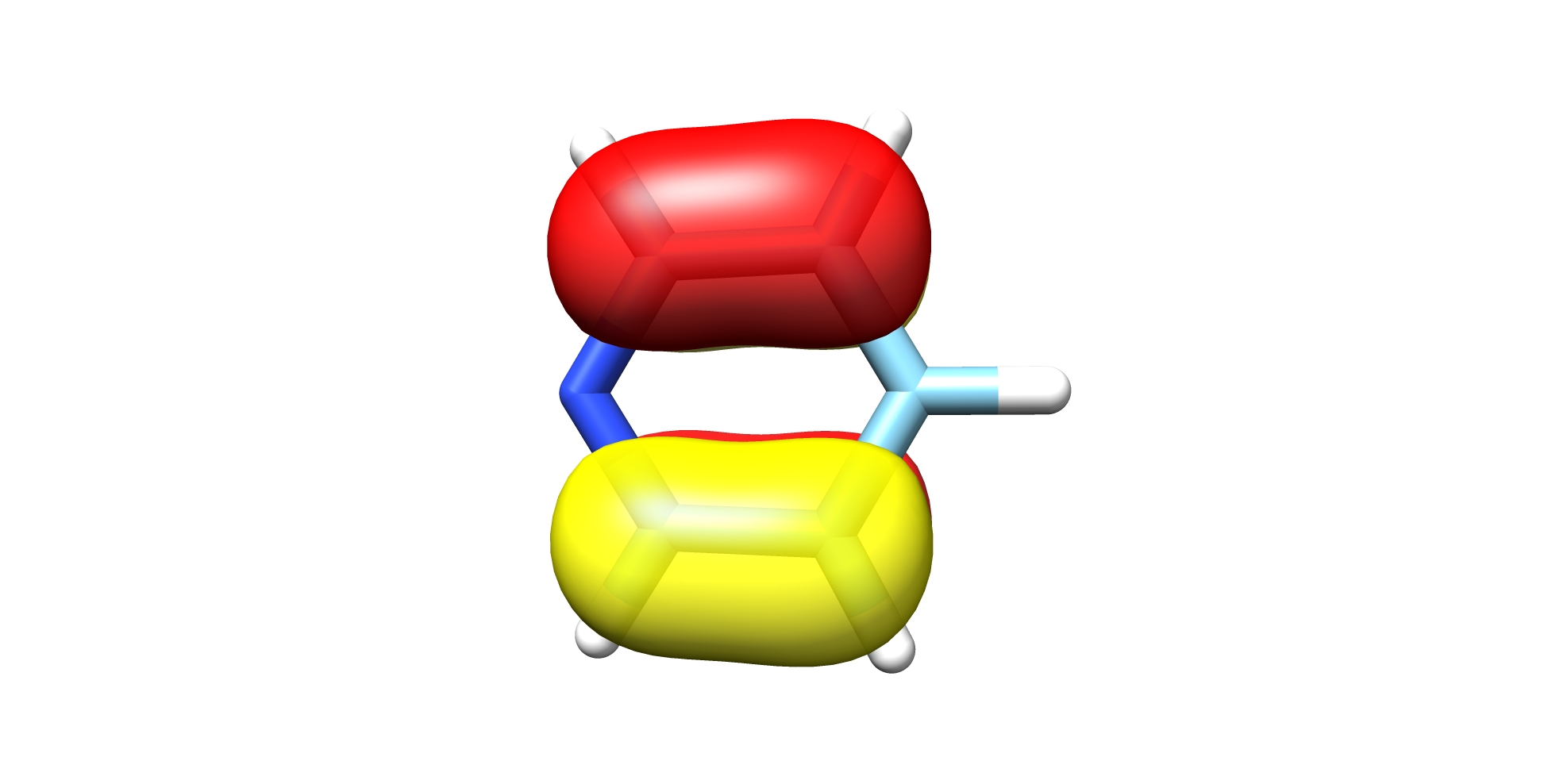
Fig. 7.66 Pyridine HOMO
7.55.7.2. List of Density Plots
If a density instead of an orbital plot is required
options 1 and 9 can be used to list the available densities.
For example option 1 in the above example will provide the
computed available densities.
Enter a number: 1
-----------------------------------------------------------------------
Reading Over   2 Saved Densities                                    ...
-----------------------------------------------------------------------
-----------------------------------------------------------------------
Plot-Type is presently: 1
-----------------------------------------------------------------------
Searching for Ground State Electron or Spin Densities:              ...
-----------------------------------------------------------------------
     1 -   molecular orbitals
     2 -   (scf) electron density                              ......  (scfp                     )  => AVAILABLE
     3 -   (scf) spin density                                  ......  (scfr                     )  - NOT AVAILABLE
     4 -   natural orbitals
     5 -   corresponding orbitals
     6 -   atomic orbitals
     7 -   mdci electron density                               ......  (mdcip                    )  - NOT AVAILABLE
     8 -   mdci spin density                                   ......  (mdcir                    )  - NOT AVAILABLE
     9 -   OO-RI-MP2 density                                   ......  (pmp2re                   )  - NOT AVAILABLE
    10 -   OO-RI-MP2 spin density                              ......  (pmp2ur                   )  - NOT AVAILABLE
    11 -   MP2 relaxed density                                 ......  (pmp2re                   )  - NOT AVAILABLE
    12 -   MP2 unrelaxed density                               ......  (pmp2ur                   )  - NOT AVAILABLE
    13 -   MP2 relaxed spin density                            ......  (rmp2re                   )  - NOT AVAILABLE
    14 -   MP2 unrelaxed spin density                          ......  (rmp2ur                   )  - NOT AVAILABLE
    15 -   LED dispersion interaction density                  ......  (ded21                    )  - NOT AVAILABLE
    16 -   Atom pair density
    17 -   Shielding Tensors
    18 -   Polarisability Tensor
    19 -   AutoCI relaxed density                              ......  (autocipre                )  - NOT AVAILABLE
    20 -   AutoCI unrelaxed density                            ......  (autocipur                )  - NOT AVAILABLE
    21 -   AutoCI relaxed spin density                         ......  (autocirre                )  - NOT AVAILABLE
    22 -   AutoCI unrelaxed spin density                       ......  (autocirur                )  - NOT AVAILABLE
In this case the (scf) electron density is available and can be chosen to be visualized in a similar process as described above for the orbitals.
Enter Type: 2
The default name of the density would be: pyridine_scf.scfp
Is this the one you want (y/n)?
While Option 9 will give us the name of this density:
---------------------
List of density names
---------------------

Index:                                                   Name of Density
------------------------------------------------------------------------
    0:                                                 pyridine_scf.scfp
Following the above steps we can visualize the SCF electron density of pyridine
PlotType       ... DENSITY-PLOT
ElDens File    ... pyridine_scf.scfp
Output file    ... MyElDens
Format         ... Grid3d/Cube
Resolution     ... 80 80 80

Calling PlotGrid3d with ATOM-A,B=0,0
Entering PlotGrid3d with Plottype =2
                 *** PLOTTING FINISHED ***
 Output file: pyridine_scf.eldens.cube
(Figure: Fig. 7.67)
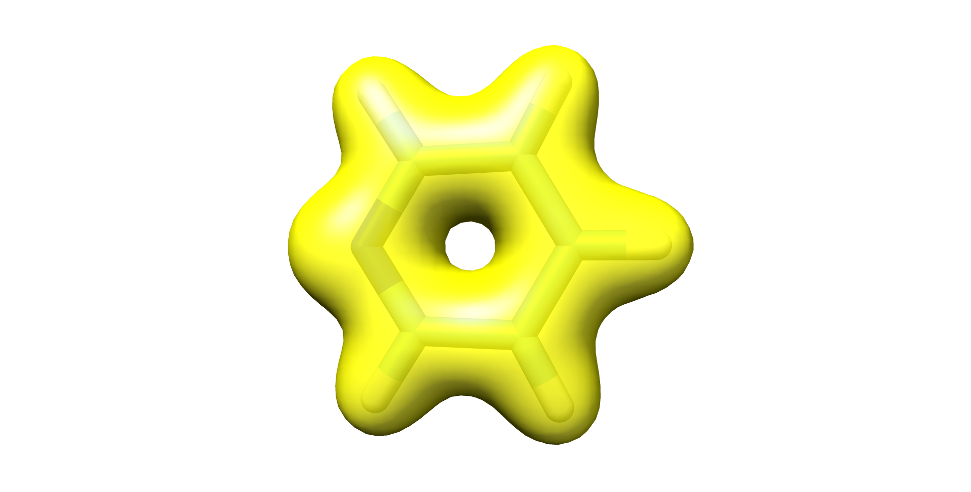
Fig. 7.67 Pyridine SCF Electron Density
7.55.7.3. Perform Algebraic Operations
Starting from ORCA 6 one can perform simple Algebraic Operations with the
computed densities. The presently available operations are listed in menu option 10:
Enter a number: 10
-----------------------------------------------------------------------
Available Algebraic Operations:
-----------------------------------------------------------------------
       1 - Pair Densities Addition
       2 - Pair Densities Subtraction
       3 - Pair Densities Multiplication
       4 - Pair Densities Division
       5 - Density Normalization
       6 - Make Natural Transition Orbitals
       7 - Make Natural Difference Orbitals
       8 - Leave Section - Return to Main Menu
The important step to these processes is to make sure that the desired
State or Transition State Densities are available in the Densities file.
To achieve this, one should request the desired densities to be stored in the disk
after the calculation is executed by the commands
!KeepDens or !KeepTransDensity. Please NOTE that storage of several
hundreds or thousands of these densities need to be done with care from
the user’s perspective as they might occupy several hundreds of GB disk space!
Let us in addition on top of the SCF calculation of pyridine perform a canonical CCSD calculation with the following input:
!CCSD def2-SVP

*xyz 0 1
C        0.690940233      0.417992301     -1.170801378
C        0.690940233      1.616339301     -0.458357378
C        0.690940233      1.560238301      0.936438622
N        0.690940233      0.417992301      1.635468622
C        0.690940233     -0.724253699      0.936438622
C        0.690940233     -0.780354699     -0.458357378
H        0.690940233      0.417992301     -2.257043378
H        0.690940233      2.574997301     -0.967574378
H        0.690940233      2.478336301      1.521602622
H        0.690940233     -1.642351699      1.521602622
H        0.690940233     -1.739012699     -0.967574378
*
Option 1 in the orca_plot menu will now provide us with both the scf and mdci
electron densities.
-----------------------------------------------------------------------
Plot-Type is presently: 1
-----------------------------------------------------------------------
Searching for Ground State Electron or Spin Densities:              ...
-----------------------------------------------------------------------
     1 -   molecular orbitals
     2 -   (scf) electron density                              ......  (scfp                     )  => AVAILABLE
     3 -   (scf) spin density                                  ......  (scfr                     )  - NOT AVAILABLE
     4 -   natural orbitals
     5 -   corresponding orbitals
     6 -   atomic orbitals
     7 -   mdci electron density                               ......  (mdcip                    )  => AVAILABLE
Hence we can proceed and in option 2 of the Available Algebraic Operations
menu take their difference to produce the respective CCSD - HF electron
correlation electron density as:
---------------------
List of density names
---------------------

Index:                                                   Name of Density
------------------------------------------------------------------------
    0:                                                pyridine_ccsd.scfp
    1:                                              pyridine_ccsd.P0.tmp
    2:                                               pyridine_ccsd.mdcip


-----------------------------------------------------------------------
Performing Algebraic Operations Over Densities: => SUBTRACTION
-----------------------------------------------------------------------
Number of Densities to be Processed from the List =>   2:
-----------------------------------------------------------------------
Enter FileName for Density[  0]: pyridine_ccsd.scfp
Provide a Scale Factor for Density[  0] (Default => 1.00): 1
Enter FileName for Density[  1]: pyridine_ccsd.mdcip
Provide a Scale Factor for Density[  1] (Default => 1.00): 1
-----------------------------------------------------------------------
INTERPRETTING EQUATION:
-----------------------------------------------------------------------
1/sqrt(N) * [(1.00) * {pyridine_ccsd.scfp} - (1.00) * {pyridine_ccsd.mdcip}]
-----------------------------------------------------------------------

PlotType       ... DENSITY-PLOT
ElDens File    ... pyridine_ccsd.scfp_minus_pyridine_ccsd.mdcip
Output file    ... pyridine_ccsd.scfp_minus_pyridine_ccsd.mdcip.cube
Format         ... Grid3d/Cube
Resolution     ... 80 80 80
We can directly visualize the produced
pyridine_ccsd.scfp_minus_pyridine_ccsd.mdcip.cube
(Figure: Fig. 7.68)
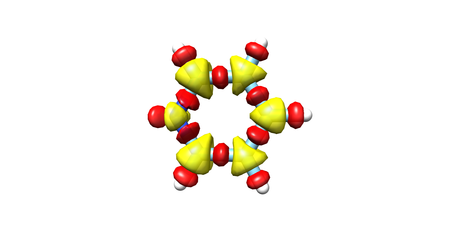
Fig. 7.68 Pyridine CCSD-HF Electron Density
NOTE: The generated density is stored in the Density Container so that it can be further processed or properly stored for future use
---------------------
List of density names
---------------------

Index:                                                   Name of Density
------------------------------------------------------------------------
    0:                                                pyridine_ccsd.scfp
    1:                                              pyridine_ccsd.P0.tmp
    2:                                               pyridine_ccsd.mdcip
    3:                      pyridine_ccsd.scfp_minus_pyridine_ccsd.mdcip
Another useful utility option of orca_plot is that is able to generate
Natural Transition Orbitals (NTOs) of Natural Difference Orbitals (NDOs)
from any theory level available State or Transition Density. Let us show case
an example. We now perform a SA-CASSCF (7,8) calculation on the pyridine molecule
according to the input where we make sure that all relevant densities are
kept on disk after the calculation by adding the KeepTransDensity in the
keyword list.
!def2-SVP KeepTransDensity

%casscf
 nel 8
 norb 7
 mult 1
 nroots 10
end


*xyz 0 1
C        0.690940233      0.417992301     -1.170801378
C        0.690940233      1.616339301     -0.458357378
C        0.690940233      1.560238301      0.936438622
N        0.690940233      0.417992301      1.635468622
C        0.690940233     -0.724253699      0.936438622
C        0.690940233     -0.780354699     -0.458357378
H        0.690940233      0.417992301     -2.257043378
H        0.690940233      2.574997301     -0.967574378
H        0.690940233      2.478336301      1.521602622
H        0.690940233     -1.642351699      1.521602622
H        0.690940233     -1.739012699     -0.967574378
*
Indeed after the calculation we now have besides the CASSCF electron densities all the relevant CASSCF State and Transition densities become now available.
-----------------------------------------------------------------------
Plot-Type is presently: 1
-----------------------------------------------------------------------
Searching for Ground State Electron or Spin Densities:              ...
-----------------------------------------------------------------------
     1 -   molecular orbitals
     2 -   (scf) electron density                              ......  (scfp                     )  => AVAILABLE
     3 -   (scf) spin density                                  ......  (scfr                     )  - NOT AVAILABLE
     ...
-----------------------------------------------------------------------
Searching for State or Transition State AO Electron Densities:      ...
-----------------------------------------------------------------------
    23 -   CIS unrelaxed transition AO density                 ......  (Tdens-CIS                )  - NOT AVAILABLE
    24 -   ROCIS unrelaxed transition AO density               ......  (Tdens-ROCIS              )  - NOT AVAILABLE
    25 -   CAS unrelaxed transition AO density                 ......  (Tdens-CAS                )  => AVAILABLE
    ...
-----------------------------------------------------------------------
Searching for State or Transition State MO Electron Densities:      ...
-----------------------------------------------------------------------
    29 -   CIS unrelaxed transition MO density                 ......  (Tdens-CISMO              )  - NOT AVAILABLE
    30 -   ROCIS unrelaxed transition MO density               ......  (Tdens-ROCISMO            )  - NOT AVAILABLE
    31 -   CAS unrelaxed transition MO density                 ......  (Tdens-CASMO              )  => AVAILABLE
   ...
We can now set ourselves to generate the NTOs and NDOs dominating the computed State 1
ROOT   1:  E=    -246.3609192216 Eh  5.176 eV  41749.8 cm**-1
      0.82391 [   346]: 2212100
      0.06447 [   295]: 2112200
Hence by using options 6 =>NTOs or 7 =>NDOs of the Available Algebraic Operations
menu, and processing the respective:
AO Transition densities \({D}_{01}\) for NTOs
-----------------------------------------------------------------------
Performing Algebraic Operations Over Densities: => MAKE_NTOS
-----------------------------------------------------------------------
Enter FileName for Density[  0]: Tdens-CAS-0-0-0-1
Provide a Scale Factor for Density[  0] (Default => 1.00): 1
-----------------------------------------------------------------------
NATURAL TRANSITION ORBITALS GENERATION:
-----------------------------------------------------------------------
Warning: The one-electron matrix doesn't exist - is recalculated (SHARK)
Calculating the overlap matrix            ... done!

------------------------------------------------
NATURAL TRANSITION ORBITALS FOR STATE     1 1A
------------------------------------------------

STATE    1 1A  :  E=   0.190226 au      5.176 eV    41749.8 cm**-1

Threshold for printing occupation numbers 1.0000e-04

     0  : n=  1.28519446
     1  : n=  0.03997952
     2  : n=  0.01505089
     3  : n=  0.00336119

=> Natural Transition Orbitals (donor   ) were saved in Tdens-CAS-0-0-0-1.1-1A_nto-donor.gbw
=> Natural Transition Orbitals (acceptor) were saved in Tdens-CAS-0-0-0-1.1-1A_nto-acceptor.gbw
-----------------------------------------------------------------------
Provide a Number of NTOs to plot (Default => 1): 1
-----------------------------------------------------------------------
-----------------------------------------------------------------------
Reading Donor NTO-file   : Tdens-CAS-0-0-0-1.1-1A_nto-donor.gbw
-----------------------------------------------------------------------
Generating cube file for Donor NTO[0]:=> Tdens-CAS-0-0-0-1.1-1A_nto-donor.gbw.0.cube
-----------------------------------------------------------------------
Reading Acceptor NTO-file   : Tdens-CAS-0-0-0-1.1-1A_nto-acceptor.gbw
-----------------------------------------------------------------------
Generating cube file for Acceptor NTO[0]:=> Tdens-CAS-0-0-0-1.1-1A_nto-acceptor.gbw.0.cube
Current-settings:

PlotType       ... MO-PLOT
MO/Operator    ... 0 0
Output file    ... Tdens-CAS-0-0-0-1.1-1A_nto-acceptor.gbw.0.cube
Format         ... Grid3d/Cube
Resolution     ... 80 80 80
AO State densities \(D_{00}-D_{11}\) for NDOs
-----------------------------------------------------------------------
Performing Algebraic Operations Over Densities: => MAKE_NDOS
-----------------------------------------------------------------------
Enter FileName for Density[  0]: Tdens-CAS-0-0-0-0
Provide a Scale Factor for Density[  0] (Default => 1.00): 1
Enter FileName for Density[  1]: Tdens-CAS-0-0-1-1
Provide a Scale Factor for Density[  1] (Default => 1.00): 1
-----------------------------------------------------------------------
NATURAL DIFFERENCE ORBITALS GENERATION:
-----------------------------------------------------------------------
Warning: The one-electron matrix doesn't exist - is recalculated (SHARK)
Calculating the overlap matrix            ... done!

------------------------------------------------
NATURAL DIFFERENCE ORBITALS FOR STATE     1 1A
------------------------------------------------

STATE    1 1A  :  E=   0.190226 au      5.176 eV    41749.8 cm**-1

Threshold for printing occupation numbers 1.0000e-04

     0  : n=  0.49881235
     1  : n=  0.08492368
     2  : n=  0.06708141
     3  : n=  0.01254920
     4  : n=  0.00667407
     5  : n=  0.00006162

=> Natural Difference Orbitals (donor   ) were saved in Tdens-CAS-0-0-0-0-Tdens-CAS-0-0-1-1.1-1A_ndo-donor.gbw
=> Natural Difference Orbitals (acceptor) were saved in Tdens-CAS-0-0-0-0-Tdens-CAS-0-0-1-1.1-1A_ndo-acceptor.gbw
-----------------------------------------------------------------------
Provide a Number of NDOs to plot (Default => 1): 1
-----------------------------------------------------------------------
-----------------------------------------------------------------------
Reading Donor NDO-file   : Tdens-CAS-0-0-0-0-Tdens-CAS-0-0-1-1.1-1A_ndo-donor.gbw
-----------------------------------------------------------------------
Generating cube file for Donor NDO[0]:=> Tdens-CAS-0-0-0-0-Tdens-CAS-0-0-1-1.1-1A_ndo-donor.gbw.0.cube
-----------------------------------------------------------------------
Reading Acceptor NDO-file   : Tdens-CAS-0-0-0-0-Tdens-CAS-0-0-1-1.1-1A_ndo-acceptor.gbw
-----------------------------------------------------------------------
Generating cube file for Acceptor NDO[0]:=> Tdens-CAS-0-0-0-0-Tdens-CAS-0-0-1-1.1-1A_ndo-acceptor.gbw.0.cube
Current-settings:

PlotType       ... MO-PLOT
MO/Operator    ... 0 0
Output file    ... Tdens-CAS-0-0-0-0-Tdens-CAS-0-0-1-1.1-1A_ndo-acceptor.gbw.0.cube
Format         ... Grid3d/Cube
Resolution     ... 80 80 80
It is possible to produce the corresponding Donor and Acceptor NTOs and NDOs orbital pairs which can be readily visualized in:
(Figure: Fig. 7.69)
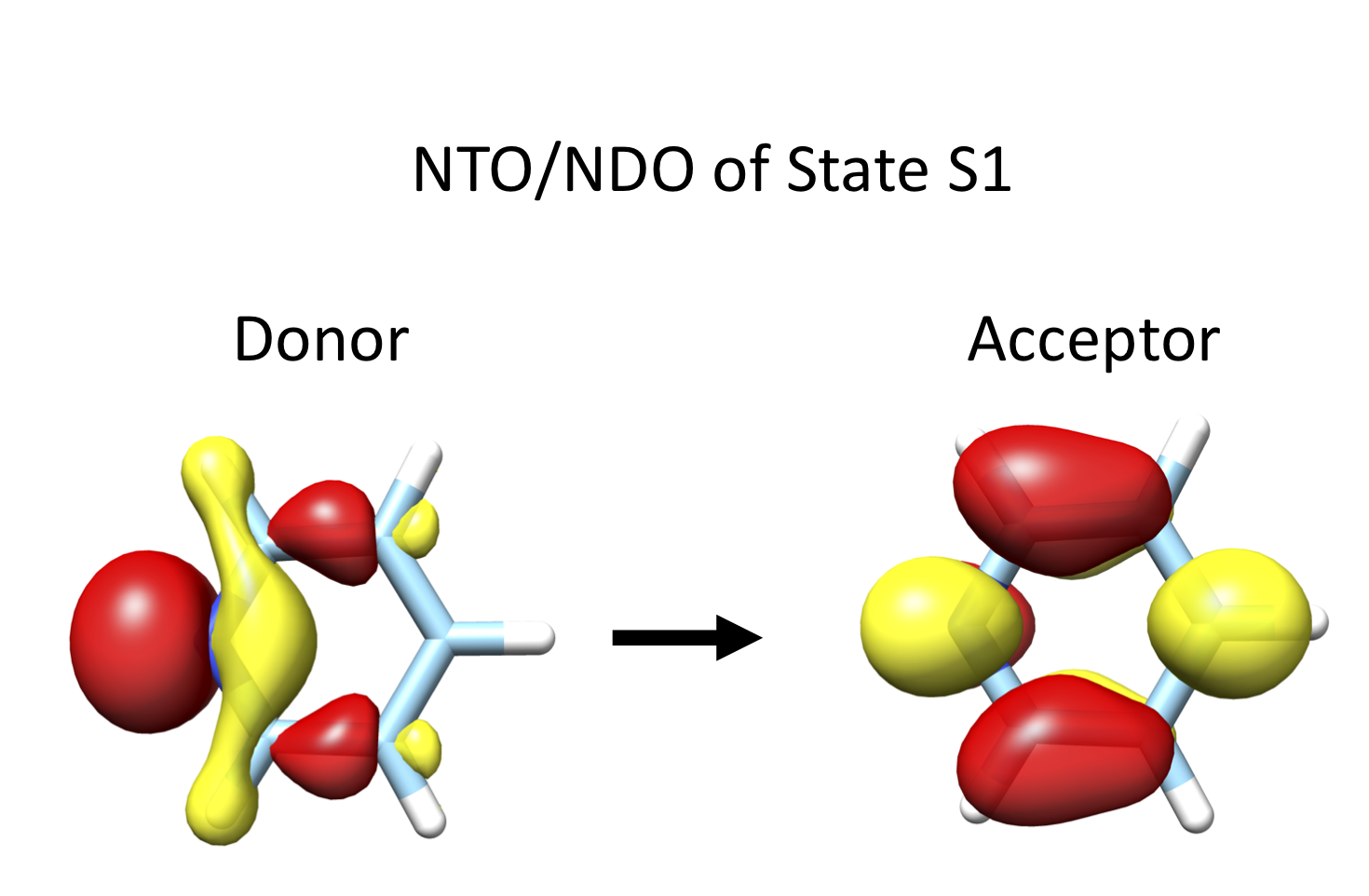
Fig. 7.69 Pyridine SA-CASSCF(8,7) NTO/NDO donor/acceptor orbital pairs for State 1
NOTE: It is beneficial and more correct to always process the AO basis Densities. In particular it is not possible nor is correct to process reduced MO basis Densities.
7.55.7.4. Additional TIPS regarding Density Plots
As an alternative to menu option
9one can check, which densities are available, directly in the calculation directory by reading out the list of all densities contained in the densities-file:
orca_plot mymol.densities
When
orca_plotis used for very expensive plots, it even can be called in parallel mode:
mpirun -np 4 /orca_path/orca_plot_mpi MyGBWFile.gbw -i MyGBWFile
It is possible to use
orca_plotto create difference densities between the ground and excited states from CIS or TD-DFT calculations directly from the .cis calculation information. This is implemented as an extra interactive menu point that is (hopefully) self-explanatory. Starting from ORCA 6 one can use theAlgebraic Operationsutility menu to carry out these operations directly from the generated State and Transition Densities.
7.55.8. orca_2mkl: Old Molekel as well as Molden inputs
This little utility program can be used to convert gbw files into mkl files which are of ASCII format. This is useful since molekel can read these files and use them for plotting and the like. The contents of the mkl file is roughly the same as the gbw file (except for the internal flags of ORCA) but this is an ASCII file which can also be read for example by your own programs. It would therefore be a good point for developing an interface. It is likely that this functionality will be further expanded in the future.
orca_2mkl BaseName
      (will produce BaseName.mkl from BaseName.gbw)
orca_2mkl BaseName -molden
      (writes a file in molden format)
orca_2mkl BaseName -mkl
      (writes a file in MKL format)
We have recently also added the capability to convert any gbw type file into MKL or Molden format. Thus, you can use this device to vizualize QRO or UNO or UCO orbitals or any type of natural orbitals:
orca_2mkl gbw_type_file.extension mkl_file.extension -mkl -anyorbs
# or
orca_2mkl gbw_type_file.extension molden_file.extension -molden -anyorbs
You also have the opportunity to run orca_2mkl backwards in order to
produce gbw type files. You can use this device in order to import
orbitals from other sources into ORCA. This is not a frequently used
option and it has limited capabilities. Hence, it is documented here
only in a cursory way in order for you to be able to experiment. Note
that the CASSCF tutorial, that supplements the manual, shows how to edit
the molecular orbitals using orca_2mkl.
orca_2mkl BaseName -gbw
      (will produce BaseName.gbw out of BaseName.mkl)
7.55.9. orca_2aim
This utility program reads a .gbw file and creates a .wfn and .wfx
file that can be used for topological analysis of the electron density
by other programs. This works for open-shell and closed-shell wave
functions. The usage is very simple – just type AIM in the simple
input line of your input file, or use
orca_2aim BaseName
      (will produce BaseName.wfn and BaseName.wfx from BaseName.gbw)
7.55.10. orca_vpot
This program calculates the electrostatic potential at a given set of user defined points. It can be used with either an input file or in interactive mode. It needs four arguments:
orca_vpot MyJob.gbw MyJob.scfp MyJob.vpot.xyz MyJob.vpot.out
First: The gbw file containing the correct geometry and basis set
Second: The desired density matrix in this basis (perhaps use the
KeepDens keyword)
Third: an ASCII file with the target positions in AU, e.g.
6                 (number_of_points)
  5.0 0.0  0.0    (XYZ coordinates)
 -5.0 0.0  0.0
  0.0 5.0  0.0
  0.0-5.0  0.0
  0.0 0.0  5.0
  0.0 0.0 -5.0
Fourth: The target file which will then contain the electrostatic potential, e.g.
6                 (number of points)
 VX1  VY1  VZ1    (potential for first point)
 VX2  VY2  VZ2    (potential for second point)
  etc.
It should be straightforward for you to read this file and use the potential for whatever purpose.
There are some special ways to call orca_vpot: A call for use in parallel mode
mpirun -np 4 /full_path/orca_vpot_mpi MyJob.gbw MyJob.scfp MyJob.pot.xyz MyJob.pot.out
A call to check, which densities are available in MyJob.densities,
orca_vpot MyJob.densities
will give you a listing of all densities contained in the file.
In the case that basename of gbw- and densities-file do not match, you have to pass the densities’ name as fifth argument to orca_vpot.
orca_vpot MyJob.gbw OtherJob.scfp MyJob.pot.xyz MyJob.pot.out OtherJob
A call to orca_vpot without any arguments will display a help message.
7.55.11. orca_euler
This utility program is used to calculate the relative orientation
between calculated hyperfine coupling (HFC)/nuclear quadrupole coupling
(NQC) tensors and a reference tensor (the calculated molecular
g-/D-tensor). The orca_euler program is run by default in an ORCA job
after the calculation of HFCs or NQCs, if g- or D-tensor are also
calculated in the same job. The utility program can also be run as a
stand-alone program. In this case the .property.txt file of a previous
NQC/HFC- and D- or g-tensor calculation must be available.
The orientation between the tensors is calculated in terms of a 3x3 rotational matrix R. This is parametrized by the three so-called Euler angles \(\alpha\), \(\beta\) and \(\gamma\). These angles define the relative orientation between two tensors A and B by three successively applied rotations around different axes in order to align A with B. In the commonly used z-y-z convention these three rotations are:
Rotate A\(_{xyz}\) counterclockwise around its \(z\) axis by \(\alpha\) to give A\(_{x'y'z'}\).
Rotate A\(_{x'y'z'}\) counterclockwise around its \(y'\) axis by \(\beta\) to give A\(_{x''y''z''}\).
Rotate A\(_{x''y''z''}\) counterclockwise around its \(z''\) axis by \(\gamma\) to align with B.
orca_euler prop-file options

  file    = basename of an ORCA .property.txt file

  options
   -refg/-refD:         Reference tensor (g-tensor or D-tensor, default is -refg)
   -conv zyz/-conv zxz: Euler rotation convention (default is zyz)
   -order:              Ordering of the reference tensor (x, y, z) with respect to
                        ORCA output (min, mid, max)
   -plotA:              plot the HFC-tensors
   -plotQ:              plot the NQC-tensors
   -detail:             print detailed information
NOTE:
By default the D-tensor is used as reference tensor only if \(S\) >\(\frac{1}{2}\) and if D>0.3 cm\(^{-1}\); in all other cases the g-tensor is used as reference tensor. The user can manually select the reference tensor – if the information is available in the prop-file – by using –
refgor -refD.By default the Euler rotation in the z-y-z convention is used. The z-x-z convention can be selected manually by using the option –
conv zxz.By default the axes of the g- or D-tensor are assigned depending on their magnitude. g\(_{\text{min} }\to g_{x}\), g\(_{\text{mid} }\to g_{y}\), g\(_{\text{max} }\to g_{z}\) (similarly for D). This ordering can be modified manually when running the standalone program as shown in the following examples:
-order 3 2 1: |
min \(\to\) z |
mid \(\to\) y |
|
max \(\to\) x |
|
-order 1 -2 3: |
min \(\to\) x |
mid \(\to\) y (flipped in the orientation) |
|
max \(\to\) z |
The nuclear hyperfine and quadrupole coupling tensors can be plotted (in the xyz-file format) by the
orca_eulerprogram using –plotAor –plotQ. The HFC tensor for atom 3 (counting starts at zero) is e.g. stored in the fileprop-file.3.A.xyz, the respective NQC tensor is stored inprop-file.3.Q.xyz. In these xyz files the position of four atoms (He, Ne, Ar, Kr) is given. The x-, y- and z-direction of the tensor are in the direction of the vectors between He-Ne, He-Ar and He-Kr.The actual definition of the used rotation matrix and more information on the relative orientation can be printed by using the option –
detail.
7.55.12. orca_exportbasis
A small utility program to print out the basis sets used by ORCA. Its
usage requires at least the name of the basis set, as specified in the
simple input line of ORCA. Additional parameters like an ECP basis set,
a list of specific atoms or the name of an ouput file are accepted. The
output is stored in ASCII format, it can be inspected and modified. The
user can choose to print the basis sets in either ORCA format, which
then can be copied into the input file, or in GAMESS-US format, which
can be read via the %basis block as externally specified basis.
NOTE: Basis set names containing special characters may need a pair
of enclosing “ or ‘ to be recognized.
USAGE: orca_exportbasis keywords options

       -b, --basis  : name of basis set
                      def2-svp
                      'def2-tzvp(-f)' - string to be passed with literals

EXAMPLE: orca_exportbasis -b svp
Additional Options:

       -e, --ecp    : ecp basis
                      sdd
                      default        - ECP-part of basis (if present)

       -f, --format : output format
                      ORCA           - to be read via %basis NewGTO
                      GAMESS-US      - to be read as %basis GTOName 'mybasis.bas'
                      default        - ORCA
       -a, --atoms  : list of elements
                      Cu             - single element
                      Ga Ge As Se    - list of elements separated by blanks
                      default        - whole periodic table is printed

       -o, --outfile: name of outputfile
                      mybasis.bas
                      default        - derived name

EXAMPLE: orca_exportbasis -b svp -e sdd -a Ag -f GAMESS-US -o mybasis.bas
The output stored in GAMESS-US format can be used in the %basis block
of the next ORCA calculation.
%basis
GTOName      "mybasis.bas"
GTOAuxJName  "myauxjbasis.bas"
GTOAuxJKName "myauxjkbasis.bas"
GTOAuxCName  "myauxjcbasis.bas"
end
7.55.13. orca_eca
This utility program makes use of the calculated exchange coupling
constants to compute relative energies of all possible spin states
through diagonalization of spin Hamiltonian. The absolute and relative
energies of the spin states are printed in the *.en and *.en0 files
respectively. The on-site spin expectation values are also printed in a
*.sp file.The following example calculates the spin ladder for a
system with exchange coupling constant of -152.48 cm**-1 between
Mn(III) and Mn(IV).
%sim
ms_bs 0.5 # Arbitrary spin state
end

# specification of spin centers
$spins 2
1 2.0  # Spin on first manganese
2 1.5  # Spin on second manganese

# Exchange coupling constant (H = -2J S1 S2)
$ecc 1
1 -152.48

$aiso_bs 2 # A false segment just to print the *.sp file
1 0.00
2 0.00
7.55.14. orca_pnmr
orca_pnmr calculates the paramagnetic contribution to the NMR
shielding tensor from EPR \(g\), \(A\), and \(D\) tensors (see Section
Paramagnetic NMR shielding tensors for theoretical
background). It is a standalone program which you can invoke on the
command line after the main ORCA calculation has finished.
Alternatively, it can read user-provided \(g\)/\(A\)/\(D\) tensors from an
input file (option -i). Note that orca_pnmr expects \(g\) and \(A\)
tensors that conform to the convention described in Section
Cartesian Index Conventions for EPR and NMR Tensors.
USAGE:    orca_pnmr BaseName [-i] [-v]

OPTIONS:  -i  : read from the input file "BaseName.pnmr.inp"
          -v  : print more output (Z matrices)
When called without options, orca_pnmr will attempt to extract \(g\),
\(D\), and \(A\) tensors from the property file BaseName.property.txt and
use these to calculate the paramagnetic shieldings at 298 K. Note that
this functionality is not sophisticated: it only recognizes EPR tensors
calculated by the EPRNMR module.
A more flexible way to use the capabilities of orca_pnmr is to manually
edit the textfile BaseName.pnmr.inp and then run orca_pnmr with the
-i option. The file has the following format:
3    # Spin multiplicity (2S+1)
298  # Temperature range minimum [K]
300  # Temperature range maximum [K]
1    # Temperature step [K]
1    # Have g-tensor? 0 or 1
  2.004689   0.000000  -0.000000 # Cartesian g-tensor
  0.000000   2.004689   0.000000 # (if available)
  0.000000   0.000000   2.002123
1    # Have D-tensor? 0 or 1
 -0.514341  -0.000000  -0.000000 # Cartesian D-tensor [cm-1]
 -0.000000  -0.514341  -0.000000 # (if available)
 -0.000000  -0.000000   1.028682
2    # Number of A-tensors
0O   # First nucleus (index,element)
-72.358765                       # Prefactor [MHz]
-78.989514   0.000000  -0.000000 # Cartesian A-tensor [MHz]
  0.000000 -78.989514  -0.000000
 -0.000000  -0.000000  53.478581
1O   # Next nucleus (index,element)
-72.358765                       # Prefactor [MHz]
-78.989516   0.000000  -0.000000 # Cartesian A-tensor [MHz]
  0.000000 -78.989516  -0.000000
 -0.000000  -0.000000  53.478580
# ... Further nuclei
\(D\) and \(g\) tensors are optional: if they are not supplied
orca_pnmrwill assume the isotropic free-electron value for \(g\), and \(D\) to be zero.\(A\) tensors, however, are not optional; without an \(A\) tensor for a given nucleus, the pNMR shielding cannot be calculated for that nucleus.
7.55.15. orca_lft
Starting from ORCA 5.0, ORCA features a standalone multiplet program called orca_lft.
Orca_lft is dedicated to experimental spectroscopists.
It is able to run an arbitrary number of spectra simulations with emphasis on X-ray spectroscopies.
In this section we briefly review the main functionalities of orca_lft. For a more detail description and examples discussion please refer to the orca_lft tutorial.
The goal is to be able to compute various spectroscopic properties of a given LFT center (ion) if one can manually pass the information of 1 and 2 electron integrals in the form of e.g the diagonal elements of the LFT matrix (LFT orbital energies) and the Slater-Condon parameters of a given LFT problem.
This will allow the experimental spectroscopist to perform a massive amount of spectra simulations during the actual running experiments
Any LFT problem can be parametrized in terms 1-electron \(H_{LF}\) matrix elements and the Slater-Condon 2-electron integrals F0, F2, F4, (or the Racah parameters A, B, C, of the d-shell). (Figure: Fig. 7.70)

Fig. 7.70 Definition of an LFT problem in terms of 1-electron energies and Slater Condon parameters (SCPs)
In practice we need to know:
the Slater Condon parameters of a given LFT problem
the \(H_{LF}\) matrix elements or the relation of them (ligand field splitting, 10Dq, AOM model)
The design workflow of orca_lft is the following:
Solve the General CI problem on a User-specified LFT problem: Type of Ion, Number of Electrons, Involved Shells, Involved Multiplicities
Compute All possible Non Relativistic States/Multiplicity
Compute the Transition Densities on the CSFs basis
Compute the Needed transition Moments in the given LFT basis (i.e. 2p3d)
Compute various properties with emphasis to X-ray spectroscopy (ABS, XAS, XES, RIXS) at the Non Relativistic Limit
Compute the respective Relativistically corrected States on the Quasi Degenerate Perturbation Theory basis
Provide access to various relativistically corrected properies (ABS, XAS, XES, RIXS, MCD, XMCD, GTensors, Dtensors, Hyperfine Couplings, Electric Field Gradients)
orca_lft requires its own input. By simply executing it from the terminal
orca_lft
one gets printings of the Usage:
************************************************************************************************************
Simulate or Fit Spectra
************************************************************************************************************

============================================================================================================
Usage: orca_lft BaseName.lft.inp [options]
============================================================================================================

------------------------------------------------------------------------------------------------------------
[Options]:
------------------------------------------------------------------------------------------------------------
-sim                          Simulate Spectra
-fit                          Fit Spectra (This is not yet availiable!)
------------------------------------------------------------------------------------------------------------

************************************************************************************************************
Generate Initial Input
************************************************************************************************************

============================================================================================================
Usage: orca_lft BaseName [options]
============================================================================================================
various Run Options:
------------------------------------------------------------------------------------------------------------
[Options]:
------------------------------------------------------------------------------------------------------------
-p_case                       Requests  p-shell case
-d_case                       Requests  d-shell case
-f_case                       Requests  f-shell case
-sp_case                      Requests sp-shell case
-ps_case                      Requests sp-shell case
-sd_case                      Requests sd-shell case
-ds_case                      Requests ds-shell case
-sf_case                      Requests sf-shell case
-fs_case                      Requests fs-shell case
-pd_case                      Requests pd-shell case
-dp_case                      Requests dp-shell case
-pf_case                      Requests pf-shell case
-fp_case                      Requests fp-shell case
-df_case                      Requests pf-shell case
-fd_case                      Requests fp-shell case
-spd_case                     Requests spd-shell case
-spf_case                     Requests spf-shell case
-sdf_case                     Requests sdf-shell case
-pdf_case                     Requests pdf-shell case
-soc                          Requests Input with SOC Constants
-atnoN                        Sets Atomic Number N
------------------------------------------------------------------------------------------------------------
-Special Cases for known Elements. LFT Parameters are filled from an internal AILFT NEVPT2 database

--------------------------------------Supported Oxidation States--------------------------------------------
Presently Default Oxidation States are supported except for Fe:
Main Elements                 -> O
TM Elements (Fe(26))          -> I,II,III
TM Elements (All other)       -> II
Lanthanide/Actinide Elements  -> III
--------------------------------------------Valence Cases---------------------------------------------------
-atnoN  -2s2p_case            Requests 2s2p-shell case for element with atomic number N (4-9)
-atnoN  -3s3p_case            Requests 3s3p-shell case for element with atomic number N (12-18)
-atnoN  -4s4p_case            Requests 4s4p-shell case for element with atomic number N (20,31-36)
-atnoN  -4s4p_case            Requests 5s5p-shell case for element with atomic number N (38,49-54)
-atnoN  -3d4s_case            Requests 3d4s-shell case for element with atomic number N (22-29)
-atnoN  -4d5s_case            Requests 4d5s-shell case for element with atomic number N (40-47)
-atnoN  -5d6s_case            Requests 4d6s-shell case for element with atomic number N (72-79)
-atnoN  -4f5d_case            Requests 4d5d-shell case for element with atomic number N (59-70)
-atnoN  -5f6d_case            Requests 5d6d-shell case for element with atomic number N (91-102)
-----------------------------------------Core-Valence Cases------------------------------------------------
-atnoN  -1s3d_case            Requests 1s3d-shell case for element with atomic number N (22-29)
-atnoN  -2p3d_case            Requests 2p3d-shell case for element with atomic number N (22-29)
-atnoN  -3p3d_case            Requests 3p3d-shell case for element with atomic number N (22-29)
--------------------------------------Core-Valence XES Cases------------------------------------------------
-atnoN  -1s2p3d_case          Requests 1s2p3d-shell case for element with atomic number N (22-29)
-atnoN  -1s3p3d_case          Requests 1s3p3d-shell case for element with atomic number N (22-29)
------------------------------------------------------------------------------------------------------------
and various Spectra Simulation Options:
************************************************************************************************************
Spectra Simulation Options for the BaseName.lft.inp:
************************************************************************************************************

------------------------------------------------------------------------------------------------------------
TIP: Switch ON a Property calculation as DoProperty true:
------------------------------------------------------------------------------------------------------------

------------------------------------------------------------------------------------------------------------
General Input Parameters:
------------------------------------------------------------------------------------------------------------
NEl                           Sets the number of electrons
Shell_PQN                     Sets the principle quantum number per type of shells (s,p,d,f)
LFTCase                       !!!ALTERNATIVE TO Shell_PQN!!! Sets the given LFT problem (2p3d, 1s3p3d, ...)
-----------------------------------------------------------------------------------------------------------
LFTCase WILL replace Shell_PQN
-----------------------------------------------------------------------------------------------------------
(e.g. Shell_PQN = 0,2,3,0 for a 2p3d calculation)
Mult                          Sets the Multiplicity/Multiplicities
NRoots                        Sets the number of Roots/Multiplicity
TMultiplets (0.01)            Threshold for the Multiplets grouping in eV
DoeV                          All values in eV. This is default. If set false the cm-1 unit is used throughout
DoRAS                         Requests a RASCI calculation
RAS(nel: m1 h/ m2 / m3 p)     Computes the X-Ray Emission Spectra

RAS-reference with nel electrons
m1= number orbitals in RAS-1
h = max. number of holes in RAS-1
m2= number of orbitals in RAS-2 (any number of electrons or holes)
m3= number of orbitals in RAS-3
p = max. number of particles in RAS-3

DoElastic                     Computes in addition the Elastic Scattering terms in RIXS/RIXSSOC calculations
------------------------------------------------------------------------------------------------------------
Non Relativistic Spectroscopic Properties:
------------------------------------------------------------------------------------------------------------
DoABS/DoXAS                   Computes the Absorption like Spectra
DoCD                          Computes the CD Spectra
DoXES                         Computes the X-Ray Emission Spectra
DoRIXS                        Computes the RIXS Spectra
DoQuadrupole                  Computes the ABS,XAS,RIXS Spectra beyond dipole approximation
------------------------------------------------------------------------------------------------------------
Relativistically Corrected Spectroscopic Properties:
------------------------------------------------------------------------------------------------------------
DoSOC                         Requests the Spin Orbit Coupling Calculations
Note that this turned on automatically if zeta SOC
constant are provided
------------------------------------------------------------------------------------------------------------
DoABS/DoXAS                   Computes the SOC Corrected Absorption like Spectra
DoCD                          Computes the SOC Corrected CD Spectra
DoMCD/DoXMCD                  Computes the SOC Corrected MCD/XMCD Spectra
DoXESSOC:                     Computes the SOC Corrected XES Spectra
DoRIXSSOC:                    Computes the SOC Corrected RIXS Spectra
DoQuadrupole                  Computes the SOC Corrected ABS,XAS, XES RIXS Spectra beyond dipole approximation
------------------------------------------------------------------------------------------------------------
Magnetic Properties:
------------------------------------------------------------------------------------------------------------
DoMagnetization               Computes the Magnetization
DoSusceptibility              Computes the Susceptibilities
DoGTensor                     Computes the g-Tensors/Matrices
DoDTensor                     Computes the Zero-Field Splittings
DoATensor                     Computes the Hyperfine Tensors
DoEFGTensor                   Computes the Electric Field Gradient Tensors
(also Moesbauer Parameters in the presence of Fe centers)
------------------------------------------------------------------------------------------------------------
Variable Parameters (if they are not given, default values are used)
------------------------------------------------------------------------------------------------------------
Temperature(300)              Temperature to be used in the SOC calculations
MagneticField(0)              Magnetic Field (in Gauss)
NPointsPsi(10)                Solid Angle Integration points Psi for MCD and XMCD
NPointsPhi(10)                Solid Angle Integration points Phi for MCD and XMCD
NPointsTheta(10)              Solid Angle Integration points Theta for MCD and XMCD
------------------------------------------------------------------------------------------------------------
Variable Parameters needed for Magnetization and Susceptibility calculations
------------------------------------------------------------------------------------------------------------
LebedevIntegrationPoints(26)  Number for Integration points for Lebedev)
LebedevPrec(5)                Precision of the grid for different field directions
(meaningful values range from 1 (smallest) to 10 (largest)
nPointsFStep (5)              Number of steps for numerical differentiation
(def: 5, meaningful values are 3, 5 7 and 9)
MAGTemperatureMIN(4.0)        Minimum Temperature (K) for Magnetization
MAGTemperatureMAX(4.0)        Maximum Temperature (K) for Magnetization
MAGTemperatureNPoints(1)      Number of Temperature points for Magnetization
MAGFieldStep(100.0)           Size of Field step for numerical differentiation (def: 100 Gauss)
MAGFieldMin(0.0)              Minimum Field (Gauss) for Magnetization
MAGFieldMax(70000.0)          Minimum Field (Gauss) for Magnetization
MAGNPoints(15)                Number of Field points for Magnetization
SUSTempMin(1)                 Minimum Temperature (K) for Susceptibility
SUSTempMxn(300.0)             Maximum Temperature (K) for Susceptibility
SUSNPoints(300)               Number of Temperature points for Susceptibility
SUSStatFieldMIN(0.0)          Minimum Static Field (Gauss) for Susceptibility
SUSStatFieldMAX(1)            Maximum Static field (Gauss) for Susceptibility
SUSStatFieldNPoints(1)        Number of Static Fields for Susceptibility
------------------------------------------------------------------------------------------------------------
Orca_lft can run standalone by processing an input file (Basename.lft.inp) with orca_lft
orca_lft BaseName.lft.inp -sim
Alternatively, one can call the main orca program like
orca BaseName.lft.inp
The different benefits of the two runs are provided in the orca_lft tutorial
Orca_lft can also be used to automatically generate initial proper input files. For example, by running
orca_lft BaseName -pd_case
will generate an initial basename.lft_pd.inp input.
-----------------------------------------------------------------
Initial Input: BaseName.lft_pd.inp for Orca_LFT has been generated:
-----------------------------------------------------------------
This will generate a bare input. One has to fill in the required LFT parameters and the desired spectroscopic properies and start the simulations like in every common multiplet program.
%lft


#-----Parameters------
NEl= 0
Shell_PQN= 0, 2, 3, 0
Mult= 0
NRoots= -1
#--------------------


#---Slater-Condon Parameters---
#---All Values in eV---
PARAMETERS
F0pp =  0.00
F2pp =  0.00
F0dd =  0.00
F2dd =  0.00
F4dd =  0.00
F0pd =  0.00
F2pd =  0.00
G1pd =  0.00
G3pd =  0.00
end
#--------------------


#---Diagonal LFT-Matrix Elelemnts---
#---All Values in eV---
FUNCTIONS
0   0 " 0.00"
1   1 " 0.00"
2   2 " 0.00"
3   3 " 0.00"
4   4 " 0.00"
5   5 " 0.00"
6   6 " 0.00"
7   7 " 0.00"
end
#--------------------


#---SPECTRA/PROPERTIES---
DoABS true
#---------
end


*xyz 0 0
Atom 0.00 0.00 0.00
*
Special initial inputs based on an internal NEVPT2 data base can also be generated. For the 2p3d LFT case of NiII this will look like this
orca_lft BaseName -atno28 -2p3d_case
------------------------------------------------------------------------------
Creating input for Atom Ni(II) ...
------------------------------------------------------------------------------

-----------------------------------------------------------------
Initial Input: BaseName.lft_pd.inp for Orca_LFT has been generated:
-----------------------------------------------------------------
This will generate the following imput where the LFT parameters are filled in from an internal NEVPT2 database from precomputed CASCI/NEVPT2 AILFT LFT parameters
In the case of \(Ni^{II}\) this will look like this. This is basically a ready to run input.
%lft


#-----Parameters------
NEl= 14
LFTCase 2p3d
Mult= 3, 1
NRoots= 25, 30
#--------------------


#---Slater-Condon Parameters---
#---All Values in eV---
PARAMETERS
F0pp =  85.88
F2pp =  54.77
F0dd =  23.31
F2dd =  13.89
F4dd =  9.14
F0pd =  33.03
F2pd =  7.76
G1pd =  6.42
G3pd =  2.11
end
#--------------------


#---Diagonal LFT-Matrix Elelemnts---
#---All Values in eV---
FUNCTIONS
0   0 " 0.00"
1   1 " 0.00"
2   2 " 0.00"
3   3 "1138.35"
4   4 "1138.35"
5   5 "1138.35"
6   6 "1138.35"
7   7 "1138.35"
end
#--------------------


#---SPECTRA/PROPERTIES---
DoABS true
#---------
end


*xyz 2 3
Ni 0.00 0.00 0.00
*
Alternatively as discussed in the Abinitio Ligand Field Theory section (1- and 2-shell Abinitio Ligand Field Theory) one may actually run a 2-shell AILFT calculation and produce the respective *nevpt2.lft.inp file
!NoIter NEVPT2 def2-SVP def2-SVP/C


%method
frozencore fc_none
end

#--------------------
#Rotate Orbitals
#--------------------
%scf
rotate
{2,6,90}
{3,7,90}
{4,8,90}
end
end

#--------------------
#General Options
#--------------------
%casscf
nel 14
norb 8
mult 3,1
nroots 100,100

LFTCase 2p3d
rel
dosoc true
end
end


*xyz 2 3
Ni      0.0000000000      0.0000000000      0.0000000000
*
The structure of an orca_lft input is the following:
It contains:
The General Parameters Block where the LFT problem is defined
—–Parameters—— NEl= 14 LFTCase 2p3d #Shells_PQN 0,2,3,0, Alternative definition using s,p,d,f main quantum numbers Mult= 3, 1 NRoots= 25, 30 ——————–
The PARAMETERS Block where the SCPs and SOC constant parameters are defined
—Slater-Condon Parameters— —All Values in eV— PARAMETERS F0pp = 85.88 F2pp = 54.77 F0dd = 23.31 F2dd = 13.89 F4dd = 9.14 F0pd = 33.03 F2pd = 7.76 G1pd = 6.42 G3pd = 2.11 end ——————–
…
—SOC-CONSTANTS— —All Values in eV— PARAMETERS ZETA_P = 10.68 ZETA_D = 0.08 end ——————–
The FUNCTIONS Block where the LFT matrix is defined
The Properties Block where the desire simulation properties are specified
—SPECTRA/PROPERTIES— DoABS true ———
The xyz Block where the ion, charge, multiplicity and coordinates (0. 0. 0.) are defined
*xyz 2 3 Ni 0.0000000000 0.0000000000 0.0000000000 *
It should be emphasized the orca_lft via the FUNCTIONS and PARAMETERS blocks provides
an arbitary paramterization of the 1-electron LFT matrix and the Slater Condon Parameters
a powerfull parameters scanability
which helps to performs any kind of simulation without any symmetry restrictions. Details regarding the use of the FUNCTIONS and PARAMETERS blocks with examples are provided in the orca_lft tutorial
Let us perform the \(Ni^{2+}\) L-edge XAS spectrum simulation using the following input
%lft


  #-----Parameters------
  NEl= 14
  LFTCase 2p3d
  Mult= 3, 1
  NRoots= 25, 30
  #--------------------


  #---Slater-Condon Parameters---
  #---All Values in eV---
  PARAMETERS
    F0pp =  85.88
    F2pp =  54.77
    F0dd =  23.31
    F2dd =  13.89
    F4dd =  9.14
    F0pd =  33.03
    F2pd =  7.76
    G1pd =  6.42
    G3pd =  2.11
  end
  #--------------------


  #---Diagonal LFT-Matrix Elelemnts---
  #---All Values in eV---
  FUNCTIONS
    0   0 " 0.00"
    1   1 " 0.00"
    2   2 " 0.00"
    3   3 "1138.35"
    4   4 "1138.35"
    5   5 "1138.35"
    6   6 "1138.35"
    7   7 "1138.35"
  end
  #--------------------

  #---SOC-CONSTANTS---
  #---All Values in eV---
  PARAMETERS
    ZETA_P = 11.341
    ZETA_D = 0.085
  end
  #--------------------

  #---SPECTRA/PROPERTIES---
  DoABS true
  DoSOC true
  #---------
end


*xyz 2 3
Ni 0.00 0.00 0.00
*
In a first step the definition of the LFT problem is performed:
------------------------------------------------------------------------------
L I G A N D    F I E L D    T H E O R Y
------------------------------------------------------------------------------


Number of electrons        = 14
Multiplicities             = 3 1
Roots                      = 25 30
Shells included            = 0 2 3 0


Definition of the ligand field basis set:
0  = pz
1  = px
2  = py
3  = dz2
4  = dxz
5  = dyz
6  = dx2y2
7  = dxy


Definition of the static ligand field by the user:
There are 9 ligand field parameters

Nr.               Name       Initial Value
-----------------------------------------
1               F0PP          85.880000
2               F2PP          54.770000
3               F0DD          23.310000
4               F2DD          13.890000
5               F4DD           9.140000
6               F0PD          33.030000
7               F2PD           7.760000
8               G1PD           6.420000
9               G3PD           2.110000


Definition of the ligand field functions by the user:
There are 8 ligand field functions

Nr.      H-element   value   function
-----------------------------------------
1   H(0,0)      0.000000000   0.00
2   H(1,1)      0.000000000   0.00
3   H(2,2)      0.000000000   0.00
4   H(3,3)   1138.350000000  1138.35
5   H(4,4)   1138.350000000  1138.35
6   H(5,5)   1138.350000000  1138.35
7   H(6,6)   1138.350000000  1138.35
8   H(7,7)   1138.350000000  1138.35


Defining the one-electron LFT matrix                     ... done
Defining the two-electron LFT matrix                     ... done
In following the CI problem is defined:
Defining the CI spaces and setting up the CI             ...
Making Checks...
Multiplicty =   3, #(configurations) =     28 #(CSF's) =     28 #(Roots) =     25
NRoots<NCSFs Adjussting  ==> (CSF's) =     25
Setting up CI...
Multiplicty =   3, #(configurations) =     28 #(CSF's) =     25 #(Roots) =     25
Making Checks...
Multiplicty =   1, #(configurations) =     36 #(CSF's) =     36 #(Roots) =     30
NRoots<NCSFs Adjussting  ==> (CSF's) =     30
Setting up CI...
Multiplicty =   1, #(configurations) =     36 #(CSF's) =     30 #(Roots) =     30
CI setup done
And the CI problem is solved:
LOWEST ROOT (ROOT 0, MULT 3) =    460.113216547 Eh 12520.317 eV

STATE ROOT MULT  DE/a.u.     DE/eV    DE/cm**-1
1:   1    3   0.000000     0.000      0.0
2:   2    3   0.000000     0.000      0.0
3:   3    3   0.000000     0.000      0.0
4:   4    3   0.000000     0.000      0.0
5:   5    3   0.000000     0.000      0.0
6:   6    3   0.000000     0.000      0.0
7:   0    1   0.086266     2.347  18933.2
8:   1    1   0.086266     2.347  18933.2
9:   2    1   0.086266     2.347  18933.2
10:   3    1   0.086266     2.347  18933.2
11:   4    1   0.086266     2.347  18933.2
12:   7    3   0.099001     2.694  21728.2
13:   8    3   0.099001     2.694  21728.2
14:   9    3   0.099001     2.694  21728.2
15:   5    1   0.132624     3.609  29107.7
16:   6    1   0.132624     3.609  29107.7
17:   7    1   0.132624     3.609  29107.7
18:   8    1   0.132624     3.609  29107.7
19:   9    1   0.132624     3.609  29107.7
20:  10    1   0.132624     3.609  29107.7
21:  11    1   0.132624     3.609  29107.7
22:  12    1   0.132624     3.609  29107.7
23:  13    1   0.132624     3.609  29107.7
24:  14    1   0.331652     9.025  72789.3
25:  15    1  29.897078   813.541 6561650.2
26:  16    1  29.897078   813.541 6561650.2
27:  17    1  29.897078   813.541 6561650.2
28:  18    1  29.897078   813.541 6561650.2
29:  19    1  29.897078   813.541 6561650.2
30:  10    3  29.915627   814.046 6565721.2
31:  11    3  29.915627   814.046 6565721.2
32:  12    3  29.915627   814.046 6565721.2
33:  13    3  29.915627   814.046 6565721.2
34:  14    3  29.915627   814.046 6565721.2
35:  15    3  29.915627   814.046 6565721.2
36:  16    3  29.915627   814.046 6565721.2
37:  17    3  29.978158   815.747 6579445.1
38:  18    3  29.978158   815.747 6579445.1
39:  19    3  29.978158   815.747 6579445.1
40:  20    3  29.978158   815.747 6579445.1
41:  21    3  29.978158   815.747 6579445.1
42:  22    3  30.016020   816.777 6587754.9
43:  23    3  30.016020   816.777 6587754.9
44:  24    3  30.016020   816.777 6587754.9
45:  20    1  30.087356   818.719 6603411.3
46:  21    1  30.087356   818.719 6603411.3
47:  22    1  30.087356   818.719 6603411.3
48:  23    1  30.106270   819.233 6607562.6
49:  24    1  30.106270   819.233 6607562.6
50:  25    1  30.106270   819.233 6607562.6
51:  26    1  30.106270   819.233 6607562.6
52:  27    1  30.106270   819.233 6607562.6
53:  28    1  30.106270   819.233 6607562.6
54:  29    1  30.106270   819.233 6607562.6
accompanied by a multiplet analysis:
---------------------------------------------------
Atomic calculation : Multiplet analysis (LFT)
---------------------------------------------------
11 multiplets found (Threshold = 0.01 eV)
0 3F | E =     0.000 eV | 2p(6)3d(8)
1 3P | E =     2.694 eV | 2p(6)3d(8)
2 3F | E =   814.046 eV | 2p(5)3d(9)
3 3D | E =   815.747 eV | 2p(5)3d(9)
4 3P | E =   816.777 eV | 2p(5)3d(9)
5 1D | E =     2.347 eV | 2p(6)3d(8)
6 1G | E =     3.609 eV | 2p(6)3d(8)
7 1S | E =     9.025 eV | 2p(6)3d(8)
8 1D | E =   813.541 eV | 2p(5)3d(9)
9 1P | E =   818.719 eV | 2p(5)3d(9)
10 1F | E =   819.233 eV | 2p(5)3d(9)
---------------------------------------------------
In following SOC is computed on the QDPT framework
*************************************
Doing QDPT with ONLY SOC!
*************************************

------------------------------------
NONZERO SOC MATRIX ELEMENTS (cm**-1)
------------------------------------

Bra                       Ket
<Block Root  S    Ms  | HSOC |  Block Root  S    Ms>    =  Real-part     Imaginary part
--------------------------------------------------------------------------------------
0    1  1.0  1.0              0     0  1.0  1.0            0.000           -685.571
0    3  1.0  1.0              0     2  1.0  1.0            0.000            342.781
0    4  1.0  1.0              0     2  1.0  1.0            0.000              0.134
0    4  1.0  1.0              0     3  1.0  1.0            0.000             -2.946
0    5  1.0  1.0              0     2  1.0  1.0            0.000              0.987
0    5  1.0  1.0              0     3  1.0  1.0            0.000              7.920
0    5  1.0  1.0              0     4  1.0  1.0            0.000          -1022.995
0    6  1.0  1.0              0     2  1.0  1.0            0.000             -3.379

...

  1   29  0.0  0.0              0    17  1.0 -1.0        -2850.628           3039.103
1   29  0.0  0.0              0    18  1.0 -1.0        -16745.172           2885.219
1   29  0.0  0.0              0    19  1.0 -1.0        -1533.311           4672.283
1   29  0.0  0.0              0    20  1.0 -1.0          105.943            -43.140
1   29  0.0  0.0              0    21  1.0 -1.0           14.076             39.149

Note: In the following the full <I|HBO+SOC|J> are printed in the CI Basis.
I,J are compound indices for |Block/Mult, Ms, Root>, where the states
are ordered first by MultBlock, then Ms and finally Root.

...
The corrected SOC states are then printed
The threshold for printing is 0.0010
Eigenvectors:
Weight      Real          Image    : Block Root    Spin   Ms
STATE   0:       0.0000
0.194318     0.035977    -0.439345 :     0    0    1    1
0.193821     0.438951     0.033797 :     0    1    1    1
0.001621    -0.008938    -0.039257 :     0    4    1    0
0.248122     0.000664    -0.498118 :     0    5    1    0
0.180615     0.034848     0.423557 :     0    0    1   -1
0.180625     0.423745    -0.032633 :     0    1    1   -1

STATE   1:       0.0000
0.180266     0.018153     0.424189 :     0    0    1    1
0.180623    -0.424680     0.016424 :     0    1    1    1
0.245822     0.492098    -0.060506 :     0    4    1    0
0.001648    -0.040383    -0.004177 :     0    5    1    0
0.002114     0.045969    -0.001038 :     0    6    1    0
0.195326     0.087330     0.433242 :     0    0    1   -1
0.192550     0.430084    -0.087049 :     0    1    1   -1

...

STATE 104: 6683223.2237
0.031604     0.157946     0.081591 :     0   17    1    1
0.054142    -0.232659    -0.003404 :     0   18    1    1
0.064958    -0.076463     0.243129 :     0   19    1    1
0.040339     0.047206     0.195219 :     0   24    1    1
0.127180    -0.000013     0.356624 :     0   20    1    0
0.001970    -0.000039    -0.044381 :     0   21    1    0
0.080521    -0.000008     0.283763 :     0   23    1    0
0.031582     0.157887    -0.081573 :     0   17    1   -1
0.054144    -0.232664     0.003379 :     0   18    1   -1
0.064929    -0.076436    -0.243078 :     0   19    1   -1
0.040357     0.047226    -0.195260 :     0   24    1   -1
0.031231    -0.176723     0.000065 :     1   21    0    0
0.376805     0.613845     0.000034 :     1   22    0    0
Followed by the SOC corrected Absorption (Here XAS) spectrum
------------------------------------------------------------------------------------------
SOC CORRECTED ABSORPTION SPECTRUM
------------------------------------------------------------------------------------------
States   Energy   Wavelength   fosc          T2       |TX|       |TY|      |TZ|
(cm-1)     (nm)                   (D**2)      (D)        (D)       (D)
------------------------------------------------------------------------------------------
0  1       0.0      0.0   0.000000000   0.00006   0.00748   0.00248   0.00014
0  2       0.0      0.0   0.000000000   0.08561   0.15114   0.25053   0.00001
0  3       0.0      0.0   0.000000000   0.08072   0.24632   0.14159   0.00001
0  4       0.0   5379590440159.6   0.000000000   0.00010   0.00622   0.00793   0.00050
0  5       0.0   5308337586647.6   0.000000000   0.00021   0.01379   0.00399   0.00008
0  6       0.0   3910043783335.5   0.000000000   0.02400   0.04644   0.14780   0.00056
0  7       0.0   3891062988270.8   0.000000000   0.03327   0.05783   0.17298   0.00064
0  8       0.0   3626963690424.4   0.000000000   0.04657   0.21455   0.02332   0.00029
0  9    1386.7   7211.2   0.000000723   0.00998   0.01613   0.09858   0.00007
0 10    1386.7   7211.2   0.000000741   0.01022   0.09943   0.01828   0.00001
0 11    1386.7   7211.2   0.000000001   0.00002   0.00200   0.00345   0.00006
0 12    1386.7   7211.2   0.000000018   0.00024   0.00512   0.01469   0.00011
0 13    1386.7   7211.2   0.000000006   0.00009   0.00899   0.00263   0.00002
0 14    1386.7   7211.2   0.000000000   0.00000   0.00044   0.00179   0.00001

...

2 101 6677152.3      1.5   0.000693465   0.00199   0.02052   0.03956   0.00095
2 102 6683223.2      1.5   0.000000000   0.00000   0.00000   0.00000   0.00000
2 103 6683223.2      1.5   0.000000000   0.00000   0.00000   0.00000   0.00000
2 104 6683223.2      1.5   0.000000000   0.00000   0.00000   0.00000   0.00000
By processing the *.out file as usual with orca_mapspc orca_mapspc the *.dat and *.stk files are generated resulting in Fig. 7.71.

Fig. 7.71 orca_lft simulated \(Ni^{2+}\) L-edge XAS spectrum
7.55.16. orca_crystalprep
ORCA 5.0 fetures a utility program that can process crystallographic files (.cif) or .xyz supercell files and produce proper inputs for the embedded cluster calculations It is named orca_crystalprep tool.
Performing an embedded cluster calculation conventionally or within the Ionic-Crystal-QMMM one needs to define basically 3 regions
The quantum cluster QC that will be treated quantum mechanically
The point charges region PC that represents the solids environment
A boundary region BR or ECP that is located between the QC and PC with the main role to prevent charge communication between the QC and PC regions.
This implies that in a first step one needs to generate a SuperCell (.xyz) structure and separate the different regions according to the calculation design. In a second step one needs to charge balance the system. All this is then need to be combined into a proper calculation input.
This is clearly a multistep and many times multiplatform process that is
Complicated
Time consuming
Not user friendly
The orca_crystalprep utility is designed to automatically generate proper inputs for ORCA embedded cluster calculations with the aim to allow to a wide range of experienaced and not experienced users the ability to setup an embedded cluster calculation with a minimal effort.
orca_crystalprep requires its own input. By simply executing it from the terminal
orca_crystalprep
one gets printings of the Usage:
************************************************************************************************************
Generate initial ORCA CrystalPrep Input
************************************************************************************************************

============================================================================================================
Usage: orca_crystalprep [Basename Input] [options]
============================================================================================================

------------------------------------------------------------------------------------------------------------
[Options]:
------------------------------------------------------------------------------------------------------------
-geninput                     Generate Initial Input
------------------------------------------------------------------------------------------------------------

************************************************************************************************************
Generate ORCA Embedding Cluster Inputs using the CrystalPrep Utility
************************************************************************************************************

============================================================================================================
Usage: orca_crystalprep [CrystalPrep Input]
============================================================================================================
and the different Options:
------------------------------------------------------------------------------------------------------------
[CrystalPrep Input Options]:
-------------------------------------------------------------------------------------------------------------
General Definitions
-------------------------------------------------------------------------------------------------------------
DoCIF                       true                     This will process a .cif file
DoXYZ                       true                     This will process a .xyz file
InputCIF                    "CIFFileName"            Set the name of the CIFFileName
InputXYZ                    "XYZFileName"            Set the name of the XYZFileName
-------------------------------------------------------------------------------------------------------------
SuperCell Construction Definitions
-------------------------------------------------------------------------------------------------------------
DoSuperCell                 true                     Flag to generate a SuperCell
SCDimension                 "axbxc"                  The Dimension of the SuperCell (e.g. "1x1x1")
InputCIF                    "CIFFileName"            Set the name of the CIFFileName
InputXYZ                    "XYZFileName"            Set the name of the XYZFileName
-------------------------------------------------------------------------------------------------------------
Embedding Cluster Definitions
-------------------------------------------------------------------------------------------------------------
DoEmbedding                  true                    Flag to generate the files for the embedding approach
UseVolumeCriterion           true                    Volume Criterion to generate layers
UseDistanceCriterion         true                    Distance Criterion to generate layers
CellVolumeFraction           value                   Cell(UniCell/SuperCell) fraction (default 1.0)
DoSimpleInput                true                    Flag to generate a conventional Embedding Cluster input
DoICQMMMInput                true                    Flag to generate a Ionic-Crystal-QMMM input
WritePDB                     true                    Flag to run a Ionic-Crystal-QMMM input from a PDF file
QCCharge                     Charge Number           Specify the total QC Charge
QCMult                       Multiplicity Number     Specify the total Multiplicity
-------------------------------------------------------------------------------------------------------------
Special Tasks on Embedding Cluster Construction/Definition
-------------------------------------------------------------------------------------------------------------
DoLayers                     true                    Request Layers Definition
1) Layers Definition. There are 2 Options:
a) The Differnt regions are build in layers as multipoles of the UnitCell
b) The Differnt regions are build in layers around a predefined QC cluster via a QCAtom List
QCLayers                     QC Layers Number        Specify the number of the QC Layers
ECPLayers                    ECP Layers Number       Specify the number of the ECP Layers
PCLayers                     PC Layers Number        Specify the number of the PC Layers
HFLayers                     HF Layers Number        Specify the number of the HF Layers
Example Input
QCLayers 1
2) Atoms Definition. This is alternative to Layers Definition (e.g. DoLayers false)
NQCAtoms                     QC Atoms  Number        Specify the number of the QC Atoms
NHFAtoms                     HF Atoms  Number        Specify the number of the HF Atoms
NECPAtoms                    ECP Atoms  Number       Specify the number of the ECP Atoms
NPCAtoms                     PC Atoms  Number        Specify the number of the PC Atoms
QCAtoms                      QC Atoms  List          Specify the List   of the QC Atoms (e.g. 0,1,4,10...
HFAtoms                      HF Atoms  List          Specify the List   of the HF Atoms (e.g. 0,1,4,10...
ECPAtoms                     ECP Atoms  List         Specify the List   of the ECP Atoms (e.g. 0,1,4,10...
PCAtoms                      PC Atoms  List          Specify the List   of the PC Atoms (e.g. 0,1,4,10...
Example Input
NQAtoms= 4
QCAtoms 0,1,4,10
-------------------------------------------------------------------------------------------------------------
Request an Explicit Atom Definion in Ionic-Crystal-QMMM
HINT: This is automatically Set to true if an Atom List (QC Atoms, ECP Atoms, ...) is provided by the user
-------------------------------------------------------------------------------------------------------------
SetQCAtoms                   true                    Set explicitely the QC Atoms
SetHFAtoms                   true                    Set explicitely the HF Atoms
SetECPAtoms                  true                    Set explicitely the ECP Atoms
SetPCAtoms                   true                    Set explicitely the PC Atoms
SetPC2Atoms                  true                    Set explicitely the PC2 Atoms
-------------------------------------------------------------------------------------------------------------
Redefine SuperCell Origin. This is for shifting the center origin to a desired atom during the SC Construction
This Helps to automatically construct desired Cluster structures using the Layers Definition
-------------------------------------------------------------------------------------------------------------
ShiftOrigin                  true                    Request Origin Shift  to a particular Atom
ChosenAtom                   an Atom Number          The Number of the Chosen atom (e.g. 2)
-------------------------------------------------------------------------------------------------------------
Neutralize the Embedded Cluster in the Simple Input
Note that in the Ionic-Crustal QMMM Input this step is taken care on demand during the QM/MM run
-------------------------------------------------------------------------------------------------------------
ChargePoints                the charge points        Specify the number of the charge points (default 1000)
ChargeStep                  the charge points        Define the step during the iterations (default 0.01)
ChargeThres                 the threshold            Define the neutralization threshold (default 0.01)
Neutralization Schemes:
NeutralizingScheme1         true                 ->  Neutralization is based on All Charges
NeutralizingScheme2         true                 ->  Neutralization is based on different charges
Equiping the ECP and PC regions
NeutralizingScheme3         true                 ->  Neutralization is based on PC2 Region
-------------------------------------------------------------------------------------------------------------
Special Definitions for the .metainfo File in the Ionic-Crustal QMMM
This helps Setting Charge/Spin in a specific atom type
It can also aid the neutralization step of the Embedded Cluster in the Simple Input
-------------------------------------------------------------------------------------------------------------
NAtomTypes                  Number of Atom Types     Specify The Atom types that will be defined
Example Input
#-------------------------
#Atom Type Charge Spin
#-------------------------
AtomTypes 2
Co    1    2.0   1.5
Co    2    3.0   0
end
This specifies the local Spin and Charge of a Td HS Co2+ center (Type 1) and a OH Co3+ center (Type 2)
During the Embedding cluster construction
-------------------------------------------------------------------------------------------------------------
In a first step the orca_crystalprep tool can be used to generate its own input. So by running:
orca_crystalprep crystalprep.inp -geninput
it will generate the following initial input:
---------------------------------------------------------------------------------
Initial Input: crystalprep.inp for Orca_CrystalPrep has been generated. All Done!
---------------------------------------------------------------------------------
which looks like the following:
%crystalprep


#************************
#Read CIF/XYZ
#************************
DoCIF true

#------------------------
#INPUT CIF/XYZ
#------------------------
#InputCIF "CIFName.cif"
#------------------------
#Set Special Tasks
#------------------------
#SpaceGroupNumber 200

#************************
#Generate SuperCell
#************************
DoSuperCell true
SCDimension "1x1x1"

#************************
#Setup Embedding Approach
#************************
DoEmbedding true
DoLayers true

#------------------------
#Atom Type Charge Spin
#------------------------
#NAtomTypes 2
#Co 1 2.0  1.5
#Co 2 3.0  0.0

#************************
#Generate Inputs
#************************
#DoSimpleInput true
#DoICQMMMInput true

#Neutralize true
#QCCharge 0
#QCMult 1
#------------------------
end
By providing names for the *.cif or *.xyz files that are desired to be processed and different options it is possible to generate a ready to run embedding cluster input as is shown in Fig. 7.72.

Fig. 7.72 Embedded cluster IC-QM/MM Input generation
For the construction of the embedded cluster structure by default a layers approach is performed in which the different structural layers are constructed as multiplets of the unitcell or a fraction of the unitcell
The unitcell fractions in terms of volume units are specified by the following keyword
CellVolumeFraction N #by default N=1
As an example let us discuss in detail the case of NaCl.
Let us assume that we want to generate an embedding cluster input
with a 20x20x20 supercell starting from the nacl.cif file
create an embedding cluster with 1 QC and 1ECPs layers
create an IC-QM/MM embedding cluster input
for this purpose the following input is used
%crystalprep


#************************
#Read CIF/XYZ
#************************
DoCIF true

#------------------------
#INPUT CIF/XYZ
#------------------------
InputCIF "nacl.cif"

#************************
#Generate SuperCell
#************************
DoSuperCell true
SCDimension "20x20x20"

#************************
#Setup Embedding Approach
#************************
DoEmbedding true
DoLayers true

#------------------------
#Atom Type Charge Spin
#------------------------
NAtomTypes 2
Na 0  1.0  0.0
Cl 1 -1.0  0.0

#************************
#Generate Inputs
#************************
DoICQMMMInput true
QCCharge 0
QCMult 1
#------------------------
end
In a first step the orca_crystalprep will process the nacl.cif file and will create the unitcell and the requested 20x20x20 supercell
-------------------------------------------------------------
Reading Information from the provided CIF file: nacl.cif
-------------------------------------------------------------

------------------------Unit Cell Parameters-----------------
Hermann-Mauguin Space Group:     P1
Space Group ID:                1
Unit Cell Symmetry:
Unit Cell Volume:             46.09
Unit Cell alpha angle:        60.00
Unit Cell beta angle:         60.00
Unit Cell gamma angle:        60.00
Unit Cell alpha length:       4.024
Unit Cell beta length:        4.024
Unit Cell gamma length:       4.024
Atom   Type   AO    x     y     z    occ
Na     0     11 0.000 0.000 0.000  1.00
Cl     1     17 0.500 0.500 0.500  1.00
Done
-------------------------------------------------------------

----------Making a SuperCell with 20x20x20 dimensions-----------
Unit Cell:
0          1          2
0       4.024000   0.000000   0.000000
1       0.000000   4.024000   0.000000
2       0.000000   0.000000   4.024000

Transformation Matrix:
0          1          2
0      80.480000   0.000000   0.000000
1       0.000000  80.480000   0.000000
2       0.000000   0.000000  80.480000


---------------------------------------------------------------------
Saving xyz file: nacl4.cif_20x20x20.xyz                   ...Done
---------------------------------------------------------------------
In a following step the costruction of the embedding cluster structure will be initiated
------------Making a Embedding Cluster Input ------------
------------Using the Layers Approach with: ------------
QC_Layers: 1
ECP_Layers: 1
PC_Layers: 1
--------------
Preparing Inputs ...
In a next step the center of the .xyz supercell will be assigned to the closest atom:
-------------------------------
The Center of XYZ Coordinates
-------------------------------
41.246, 41.246, 41.246
-------------------------------
Closest Atom to Center
-------------------------------
Na(4630) 40.240, 40.240, 40.240
-------------------------------
Shifting Origin to closest atom
-------------------------------
40.240, 40.240, 40.240
In following an automatic layers generation is performed
--------------------------------------
Saving Generated Layers XYZ Files ...
--------------------------------------
Saving Layer 0 XYZ File: nacl.cif_20x20x20.xyz_0.xyz
Saving Layer 1 XYZ File: nacl.cif_20x20x20.xyz_1.xyz
Saving Layer 2 XYZ File: nacl.cif_20x20x20.xyz_2.xyz
Saving Layer 3 XYZ File: nacl.cif_20x20x20.xyz_3.xyz
Saving Layer 4 XYZ File: nacl.cif_20x20x20.xyz_4.xyz
Saving Layer 5 XYZ File: nacl.cif_20x20x20.xyz_5.xyz
Saving Layer 6 XYZ File: nacl.cif_20x20x20.xyz_6.xyz
Saving Layer 7 XYZ File: nacl.cif_20x20x20.xyz_7.xyz
Saving Layer 8 XYZ File: nacl.cif_20x20x20.xyz_8.xyz
Saving Layer 9 XYZ File: nacl.cif_20x20x20.xyz_9.xyz

--------------------------------------
Saving Generated Layers PDB File ...
--------------------------------------
The embedding cluster is then constructed:
--------------------------------------
Saving Generated Cluster XYZ Files ...
--------------------------------------
Saving QC XYZ File: nacl.cif_20x20x20.xyz_QC.xyz
Saving ECP Region XYZ File: nacl.cif_20x20x20.xyz_ECP.xyz
Saving PC Region XYZ File: nacl.cif_20x20x20.xyz_PC.xyz
Finally the IC-QM/MM embedding cluster will be generated
--------------------------------------
Saving Embedding Cluster Inputs ...
--------------------------------------
Saving ICQMMM Input: nacl.cif_20x20x20.xyz.ICQMMM.inp
Done
--------------------------------------------------------------
Ionic-Crystal QM/MM requires the generation of a simple force field *.prms For details see section: ORCA Multiscale Implementation The needed information including charge and spin is taken from a *metainfo file. The orca_crystalprep provides the possibility to externally set chatge and spin in the *.metainfo file
This is acheived by the following process:
At first processing of the .cif files assignes atom types to all the detected atoms in the asymetric unit
Atom   Type   AO    x     y     z    occ
Na     0     11 0.000 0.000 0.000  1.00
Cl     1     17 0.500 0.500 0.500  1.00
In the orca_crystalprep input it is possible to assign specific initial charge and spin to atoms of a paricular atom type in the following way:
NAtomTypes 2
Na 0  1.0  0.0
Cl 1 -1.0  0.0
This information is then passed in the *.metainfo file
18522
# atom nr. - element - atom type - formal charge - formal spin - molecule nr
0  Na   0  1  0           1
1  Na   0  1  0           1
2  Na   0  1  0           1
...

9261  Cl   1 -1  0        1
9262  Cl   1 -1  0        1
9263  Cl   1 -1  0        1
...
The constructed embedded cluster is shown in Fig. 7.73.

Fig. 7.73 Generated Embedded cluster. QC: \({Na_4}{Cl_4}\), ECP region red dots, PC region small green and purple dots
while the generated IC-QM/MM embeding cluster input is provided below
!Ionic-Crystal-QMMM
#Include Method
%qmmm
#--------Define the Cluster---------
ORCAFFFilename= ""
Use_QM_InfoFromPDB true
Use_QM3_InfoFromPDB true
ECPLayerECP= "SDD"
#--------Charge Convergence---------
CONV_Charges false
ENFORCETOTALCHARGE true
CHARGE_TOTAL    0
PrintLevel 4
end
#-----------------------------------

*pdbfile 0  1 nacl.cif_20x20x20.pdb
Note: that the information regarding the QC, ECP and PC regions is read from the generated *.pdb file
Further information regarding the IC-QM/MM and the QM/MM module in general is provided in section ORCA Multiscale Implementation
Further information and examples regarding the orca_crystalprep tool and the embedding approach is provided in the Treating Solids with the Embedding Cluster approach tutorial.