6.3. Geometry Optimizations, Surface Scans, Transition States, MECPs, Conical Intersections, IRC, NEB
The usage of analytic gradients is necessary for efficient geometry optimization. In ORCA 5.0, the following methods provide analytic first derivatives
Hartree-Fock (HF) and DFT (including the RI, RIJK and RIJCOSX approximations)
MP2, RI-MP2 and DLPNO-MP2
TD-DFT for excited states
CAS-SCF
When the analytic gradients are not available, it is possible to evaluate the first derivatives numerically by finite displacements. This is available for all methods.
The coordinate system chosen for geometry optimization affects the convergence rate, with redundant internal coordinates being usually the best choice.
Some methods for locating transition states (TS) require second derivative matrices (Hessian), implemented analytically for HF, DFT and MP2. Additionally, several approaches to construct an initial approximate Hessian for TS optimization are available. A very useful feature for locating complicated TSs is the Nudged-Elastic Band method in combination with the TS finding algorithm (NEB-TS, ZOOM-NEB-TS). An essential feature for chemical processes involving excited states is the conical intersection optimizer. Another interesting feature are MECP (Minimum Energy Crossing Point) optimizations.
For very large systems ORCA provides a very efficient L-BFGS optimizer, which makes use of the orca_md module. It can also be invoked via simple keywords described at the end of this section.
6.3.1. Geometry Optimizations
Optimizations are fairly easy as in the following example:
! B3LYP/G SV(P) Opt
* int 0 1
    C  0 0 0 0.0000   0.000    0.00
    O  1 0 0 1.2029   0.000    0.00
    H  1 2 0 1.1075 122.016    0.00
    H  1 2 3 1.1075 122.016  180.00
*
An optimization with the RI method (the BP functional is recommend) would simply look like:
! BP SV(P) OPT
* int 0 1
    C  0 0 0 0.0000   0.000    0.00
    O  1 0 0 1.2029   0.000    0.00
    H  1 2 0 1.1075 122.016    0.00
    H  1 2 3 1.1075 122.016  180.00
*
An optimization of the first excited state of ethylene:
! BLYP SVP OPT

%tddft
   IRoot 1
end

* xyz 0 1
 C     0.000000     0.000000     0.666723
 C     0.000000     0.000000    -0.666723
 H     0.000000    -0.928802     1.141480
 H    -0.804366    -0.464401    -1.341480
 H     0.000000     0.928802     1.241480
 H     0.804366     0.464401    -1.241480
*
6.3.2. Numerical Gradients
If the analytic gradient is not available, the numerical gradient can simply be requested via:
! NumGrad
as in the following example:
!CCSD(T) TZVPP
!Opt NumGrad
* int 0 1
C 0 0 0  0   0   0
O 1 0 0  1.2 0   0
H 1 2 0  1.1 120 0
H 1 2 3  1.1 120 180
*
NOTE
Be aware that the numerical gradient is quite expensive. The time for one gradient calculation is equal to 6 \(\times\) (number of atoms) \(\times\) (time for one single point calculation).
The numerical gradient can be calculated in a multi-process run, using a maximum of three times the number of atoms (see section Calling the Program with Multiple Processes).
More details on various options, geometry convergence criteria and the like are found in section Geometry Optimization.
6.3.3. Some Notes and Tricks
Note
TightSCFin the SCF part is set as default to avoid the buildup of too much numerical noise in the gradients.Even if the optimization does not converge, the ORCA output may still end with “****ORCA TERMINATED NORMALLY****”. Therefore do not rely on the presence of this line as an indicator of whether the geometry optimization is converged! Rather, one should instead rely on the fact that, an optimization job that terminates because the maximum number of iterations has been reached, will generate the following output message:
Warning
   The optimization did not converge but reached the maximum number of
   optimization cycles. Please check your results very carefully.
While a successfully converged job will generate the following message instead:
***********************HURRAY********************
***        THE OPTIMIZATION HAS CONVERGED     ***
*************************************************
Tip
In rare cases the redundant internal coordinate optimization fails. In this case, you may try to use
COPT(optimization in Cartesian coordinates). This will likely take many more steps to converge but should be stable.For optimizations in Cartesian coordinates the initial guess Hessian is constructed in internal coordinates and thus these optimizations should converge only slightly slower than those in internal coordinates. Nevertheless, if you observe a slow convergence behaviour, it may be a good idea to compute a Hessian initially (perhaps at a lower level of theory) and use
InHess readin order to improve convergence.At the beginning of a TS optimization more information on the curvature of the PES is needed than a model Hessian can give. The best choice is analytic Hessian, available for HF, DFT and MP2. In other cases (e.g. CAS-SCF), the numerical evaluation is necessary. Nevertheless you do not need to calculate the full Hessian when starting such a calculation. With ORCA we have good experience with approximations to the exact Hessian. Here it is recommended to either directly combine the TS optimization with the results of a relaxed surface scan or to use the Hybrid Hessian as the initial Hessian, depending on the nature of the TS mode. Note that these approximate Hessians do never replace the exact Hessian at the end of the optimization, which is always needed to verify the minimum or first order saddle point nature of the obtained structure.
6.3.4. Initial Hessian for Minimization
The convergence of a geometry optimization crucially depends on the
quality of the initial Hessian. In the simplest case it is taken as a
unit matrix (in redundant internal coordinates we use 0.5 for bonds, 0.2
for angles and 0.1 for dihedrals and improper torsions). However, simple
model force-fields like the ones proposed by Schlegel, Lindh, Swart or
Almlöf are available and lead to much better convergence. The different
guess Hessians can be set via the InHess option which can be either
unit, Almloef, Lindh, Swart or Schlegel in redundant internal
coordinates. Since version 2.5.30, these model force-fields (built up in
internal coordinates) can also be used in optimizations in Cartesian
coordinates.
For minimizations we recommend the Almloef Hessian, which is the
default for minimizations. The Lindh and Schlegel Hessian yield a
similar convergence behaviour. From version 4.1?, there is also the
option for the Swart model Hessian, which is less parametrized and
should improve for weakly interacting and/or unusual structures. Of
course the best Hessian is the exact one. Read may be used to input an
exact Hessian or one that has been calculated at a lower level of theory
(or a “faster” level of theory). From version 2.5.30 on this option is
also available in redundant internal coordinates. But we have to point
out that the use of the exact Hessian as initial one is only of little
help, since in these cases the convergence is usually only slightly
faster, while at the same time much more time is spent in the
calculation of the initial Hessian.
To sum it up: we advise to use one of the simple model force-fields for minimizations.
6.3.5. Coordinate Systems for Optimizations
The coordinate system for the optimization can be chosen by the
coordsys variable that can be set to cartesian or redundantwithin
the %geom block. The default is the redundant internal coordinate
system. If the optimization with redundant fails, you can still try
cartesian. If the optimization is then carried out in Cartesian
displacement coordinates with a simple model force-field Hessian, the
convergence will be only slightly slower. With a unit matrix initial
Hessian very slow convergence will result.
A compound job two_step_opt.inp that first computes a semi-empirical
Hessian to start from is shown below:
* int 0 1
C 0 0 0 0 0 0
O 1 0 0 1.3 0 0
H 1 2 0 1.1 110 0
H 1 2 3 1.1 110 180
*

%compound
# Step 1: semiempirical calculation of the Hessian
New_Step
! AM1 NumFreq
Step_End

# Step 2: optimization starting from previous Hessian
New_Step
!B3LYP def2-svp def2/J Opt
%geom
InHess
 Read
InHessName "two_step_opt_Compound_1.hess"
# this file must be either a .hess file from a
# frequency run or, a .opt/.carthess file left over from a
# previous geometry optimization
end
Step_End

End
Tip
For transition metal complexes MNDO, AM1 or PM3 Hessians are not available. You can use ZINDO/1 or NDDO/1 Hessians instead. They are of lower quality than MNDO, AM1 or PM3 for organic molecules but they are still far better than the standard unit matrix choice.
If the quality of the initial semi-empirical Hessian is not sufficient you may use a “quick” RI-DFT job (e.g.
BP def2-sv(p) defgrid1)In semi-empirical geometry optimizations on larger molecules or in general when the molecules become larger the redundant internal space may become large and the relaxation step may take a significant fraction of the total computing time.
For condensed molecular systems and folded molecules (e.g. a U-shaped carbon chain) atoms can get very close in space, while they are distant in terms of number of bonds connecting them. As damping of optimization steps in internal coordinates might not work well for these cases, convergence can slow down. ORCA’s automatic internal coordinate generation takes care of this problem by assigning bonds to atom pairs that are close in real space, but distant in terms of number of bonds connecting them.
%geom
 AddExtraBonds true         # switch on/off assigning bonds to atom pairs that are
                            #  connected by more than <Max_Length> bonds and are less
                            #  than <MaxDist> Ang. apart (default true)
 AddExtraBonds_MaxLength 10 # cutoff for number of bonds connecting the two
                            #  atoms (default 10)
 AddExtraBonds_MaxDist 5    # cutoff for distance between two atoms (default 5 Ang.)
end
For solid systems modeled as embedded solids the automatically generated set of internal coordinates might become very large, rendering the computing time spent in the optimization routine unnecessarily large. Usually, in such calculations the cartesian positions of outer atoms, coreless ECPs and point charges are constrained during the optimization - thus most of their internal coordinates are not needed. By requesting:
%geom
 ReduceRedInts true
 end
only the required needed internal coordinates (of the constrained atoms) are generated.
OBS: If the step in redundant fails badly and only Cartesian
constrains are set (or no constrains), ORCA will fallback to a
cartesian step automatically. This can be turned off by setting
CARTFALLBACK to FALSE.
6.3.6. Constrained Optimizations
You can perform constrained optimizations which can, at times, be extremely helpful. This works as shown in the following example:
! RKS B3LYP/G SV(P) Opt
%geom Constraints
        { B 0 1 1.25 C }
        { A 2 0 3 120.0 C }
        end
      end

* int 0 1
    C  0 0 0 0.0000   0.000    0.00
    O  1 0 0 1.2500   0.000    0.00
    H  1 2 0 1.1075 122.016    0.00
    H  1 2 3 1.1075 122.016  180.00
*
Constraining bond distances        :   { B N1 N2 value C }
Constraining bond angles           :   { A N1 N2 N1 value C }
Constraining dihedral angles       :   { D N1 N2 N3 N4 value C }
Constraining cartesian coordinates :   { C N1 C }
Note
Like for normal optimizations you can use numerical gradients (see Numerical Gradients.) for constrained optimizations. In this case the numerical gradient will be evaluated only for non-constrained coordinates, saving a lot of computational effort, if a large part of the structure is constrained.
“value” in the constraint input is optional. If you do not give a value, the present value in the structure is constrained. For cartesian constraints you can’t give a value, but always the initial position is constrained.
It is recommended to use a value not too far away from your initial structure.
It is possible to constrain whole sets of coordinates:
all bond lengths where N1 is involved       : { B N1 * C}
all bond lengths                            : { B * * C}
all bond angles where N2 is the central atom: { A * N2 * C }
all bond angles                             : { A * * * C }
all dihedral angles with central bond N2-N3 : { D * N2 N3 * C }
all dihedral angles                         : { D * * * * C }
For Cartesian constraints lists of atoms can be defined:
a list of atoms (10 to 17) with Cartesian constraints : { C 10:17 C}
Coordinates along a single Cartesian direction can be frozen as described in section Special definitions.
If there are only a few coordinates that have to be optimized you can use the
invertConstraintsoption:
%geom Constraints
        { B 0 1 C }
        end
      invertConstraints true # only the C-O distance is optimized
                             # does not affect Cartesian coordinates
      end
In some cases it is advantageous to optimize only the positions of the hydrogen atoms and let the remaining molecule skeleton fixed:
%geom optimizehydrogens true
      end
Note
In the special case of a fragment optimization (see next point) the
optimizehydrogenskeyword does not fix the heteroatoms, but ensures that all hydrogen positions are relaxed.In Cartesian optimization, only Cartesian constraints are allowed.
6.3.7. Constrained Optimizations for Molecular Clusters (Fragment Optimization)
If you want to study systems, which consist of several molecules (e.g. the active site of a protein) with constraints, then you can either use cartesian constraints (see above) or use ORCA’s fragment constraint option. ORCA allows the user to define fragments in the system. For each fragment one can then choose separately whether it should be optimized or constrained. Furthermore, it is possible to choose fragment pairs whose distance and orientation with respect to each other should be constrained. Here, the user can either define the atoms which make up the connection between the fragments, or the program chooses the atom pair automatically via a closest distance criterion. ORCA then chooses the respective constrained coordinates automatically. An example for this procedure is shown below.
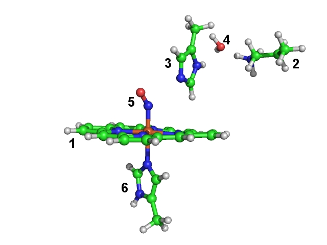
The coordinates are taken from a crystal structure [PDB-code 2FRJ]. In our gas phase model we choose only a small part of the protein, which is important for its spectroscopic properties. Our selection consists of a heme-group (fragment 1), important residues around the reaction site (lysine (fragment 2) and histidine (fragment 3)), an important water molecule (fragment 4), the NO-ligand (fragment 5) and part of a histidine (fragment 6) coordinated to the heme-iron. In this constrained optimization we want to maintain the position of the heteroatoms of the heme group. Since the protein backbone is missing, we have to constrain the orientation of lysine and histidine (fragments 2 and 3) side chains to the heme group. All other fragments (the ones which are directly bound to the heme-iron and the water molecule) are fully optimized internally and with respect to the other fragments. Since the crystal structure does not reliably resolve the hydrogen positions, we relax also the hydrogen positions of the heme group.
# !! If you want to run this optimization: be aware
# !!  that it will take some time!
! BP86 SV(P) Opt
%geom
    ConstrainFragments { 1 } end # constrain all internal
                                 # coordinates of fragment 1
    ConnectFragments
     {1 2 C 12 28}  # connect the fragments via the atom pair 12/28 and 15/28 and
     {1 3 C 15 28}  #  constrain the internal coordinates connecting
                    #  fragments 1/2 and 1/3
      {1 5 O}
      {1 6 O}
      {2 4 O}
      {3 4 O}
    end
    optimizeHydrogens true  # do not constrain any hydrogen position
  end
* xyz 1 2
Fe(1)     -0.847213     -1.548312     -1.216237 newgto "TZVP" end
 N(5)     -0.712253     -2.291076      0.352054 newgto "TZVP" end
 O(5)     -0.521243     -3.342329      0.855804 newgto "TZVP" end
 N(6)     -0.953604     -0.686422     -3.215231 newgto "TZVP" end
 N(3)     -0.338154     -0.678533      3.030265 newgto "TZVP" end
 N(3)     -0.868050      0.768738      4.605152 newgto "TZVP" end
 N(6)     -1.770675      0.099480     -5.112455 newgto "TZVP" end
 N(1)     -2.216029     -0.133298     -0.614782 newgto "TZVP" end
 N(1)     -2.371465     -2.775999     -1.706931 newgto "TZVP" end
 N(1)      0.489683     -2.865714     -1.944343 newgto "TZVP" end
 N(1)      0.690468     -0.243375     -0.860813 newgto "TZVP" end
 N(2)      1.284320      3.558259      6.254287
 C(2)      5.049207      2.620412      6.377683
 C(2)      3.776069      3.471320      6.499073
 C(2)      2.526618      2.691959      6.084652
 C(3)     -0.599599     -0.564699      6.760567
 C(3)     -0.526122     -0.400630      5.274274
 C(3)     -0.194880     -1.277967      4.253789
 C(3)     -0.746348      0.566081      3.234394
 C(6)      0.292699      0.510431     -6.539061
 C(6)     -0.388964      0.079551     -5.279555
 C(6)      0.092848     -0.416283     -4.078708
 C(6)     -2.067764     -0.368729     -3.863111
 C(1)     -0.663232      1.693332     -0.100834
 C(1)     -4.293109     -1.414165     -0.956846
 C(1)     -1.066190     -4.647587     -2.644424
 C(1)      2.597468     -1.667470     -1.451465
 C(1)     -1.953033      1.169088     -0.235289
 C(1)     -3.187993      1.886468      0.015415
 C(1)     -4.209406      0.988964     -0.187584
 C(1)     -3.589675     -0.259849     -0.590758
 C(1)     -3.721903     -2.580894     -1.476315
 C(1)     -4.480120     -3.742821     -1.900939
 C(1)     -3.573258     -4.645939     -2.395341
 C(1)     -2.264047     -4.035699     -2.263491
 C(1)      0.211734     -4.103525     -2.488426
 C(1)      1.439292     -4.787113     -2.850669
 C(1)      2.470808     -3.954284     -2.499593
 C(1)      1.869913     -2.761303     -1.932055
 C(1)      2.037681     -0.489452     -0.943105
 C(1)      2.779195      0.652885     -0.459645
 C(1)      1.856237      1.597800     -0.084165
 C(1)      0.535175      1.024425     -0.348298
 O(4)     -1.208602      2.657534      6.962748
 H(3)     -0.347830     -1.611062      7.033565
 H(3)     -1.627274     -0.387020      7.166806
 H(3)      0.121698      0.079621      7.324626
 H(3)      0.134234     -2.323398      4.336203
 H(3)     -1.286646      1.590976      5.066768
 H(3)     -0.990234      1.312025      2.466155
 H(4)     -2.043444      3.171674      7.047572
 H(2)      1.364935      4.120133      7.126900
 H(2)      0.354760      3.035674      6.348933
 H(2)      1.194590      4.240746      5.475280
 H(2)      2.545448      2.356268      5.027434
 H(2)      2.371622      1.797317      6.723020
 H(2)      3.874443      4.385720      5.867972
 H(2)      3.657837      3.815973      7.554224
 H(2)      5.217429      2.283681      5.331496
 H(2)      5.001815      1.718797      7.026903
 H(6)     -3.086380     -0.461543     -3.469767
 H(6)     -2.456569      0.406212     -5.813597
 H(6)      1.132150     -0.595619     -3.782287
 H(6)      0.040799      1.559730     -6.816417
 H(6)      0.026444     -0.139572     -7.404408
 H(6)      1.392925      0.454387     -6.407850
 H(1)      2.033677      2.608809      0.310182
 H(1)      3.875944      0.716790     -0.424466
 H(1)      3.695978     -1.736841     -1.485681
 H(1)      3.551716     -4.118236     -2.608239
 H(1)      1.487995     -5.784645     -3.308145
 H(1)     -1.133703     -5.654603     -3.084826
 H(1)     -3.758074     -5.644867     -2.813441
 H(1)     -5.572112     -3.838210     -1.826943
 H(1)     -0.580615      2.741869      0.231737
 H(1)     -3.255623      2.942818      0.312508
 H(1)     -5.292444      1.151326     -0.096157
 H(1)     -5.390011     -1.391441     -0.858996
 H(4)     -1.370815      1.780473      7.384747
 H(2)      5.936602      3.211249      6.686961
*
Note
You have to connect the fragments in such a way that the whole system is connected.
You can divide a molecule into several fragments.
Since the initial Hessian for the optimization is based upon the internal coordinates: Connect the fragments in a way that their real interaction is reflected.
This option can be combined with the definition of constraints, scan coordinates and the
optimizeHydrogensoption (but: its meaning in this context is different to its meaning in a normal optimization run, relatively straightforward see section Geometry Optimization).Can be helpful in the location of complicated transition states (with relaxed surface scans).
6.3.8. Adding Arbitrary Wall Potentials
For some applications, it might be interesting to add arbitrary wall potentials during the geometry optimization. For example, if you want to optimize an intermolecular complex and need that both structures stick together, without one flying away during the optimization, or when using microsolvation.
In ORCA you can add three kinds of arbitrary “wall potentials”: an ellipsoid or spherical of the form
or a rectangular box potential with 6 walls of the form
These can be given in two ways: by explicitly defining the origin of the potential and its limits, e.g:
%GEOM ELLIPSEPOT 0,0,0,5,3,4 # the last are the a,b and c radii
or:
%GEOM SPHEREPOT 0,0,0,5 # the last is the radius
or:
%GEOM BOXPOT 0,0,0,4,-4,3,-3,6,-6 # maxx, minx, maxy, miny, maxz and minz last
where the first three numbers are the center and the last is the radius for the sphere (or a,b and c for the ellipsoid) and the max and min x,y and z dimensions of the box. All numbers should be given in Ångström.
In case a single number is given instead, the walls will be automatically centered around the centroid of the molecule and that number will be added to the minimum sphere or box that is necessary to contain the molecule. For example:
%GEOM SPHEREPOT 2
or:
%GEOM BOXPOT 2
will build a minimum wall centered on the centroid that encloses the molecule and add 2 Ångström on top of it. Still on the sphere case, a negative number like
%GEOM SPHEREPOT -2
will make the total radius of the sphere to be Ångström.
OBS: This will apply to regular geometry optimizations, as well as to the Global Optimizer (GOAT).
6.3.9. Relaxed Surface Scans
A final thing that comes in really handy are relaxed surface scans, i.e. you can scan through one coordinate while all others are relaxed. It works as shown in the following example:
! B3LYP/G SV(P) Opt
%geom Scan
        B 0 1 = 1.35, 1.10, 12 # C-O distance that will be scanned
        end
      end

* int 0 1
    C  0 0 0 0.0000   0.000    0.00
    O  1 0 0 1.3500   0.000    0.00
    H  1 2 0 1.1075 122.016    0.00
    H  1 2 3 1.1075 122.016  180.00
*
In the example above the value of the bond length between C and O will be changed in 12 equidistant steps from 1.35 down to 1.10 Ångströms and at each point a constrained geometry optimization will be carried out.
Note
If you want to perform a geometry optimization at a series of values with non-equidistant steps you can give this series in square brackets, [ ]. The general syntax is as follows:
B N1 N2 = initial-value, final-value, NSteps
or:
B N1 N2 [value1 value2 value3 ... valueN]
In addition to bond lengths you can also scan bond angles and dihedral angles:
B N1 N2 = ...              # bond length
A N1 N2 N3 = ...           # bond angle
D N1 N2 N3 N4 = ...        # dihedral angle
Tip
As in constrained geometry optimizations it is possible to start the relaxed surface scan with a different scan parameter than the value present in your molecule. But keep in mind that this value should not be too far away from your initial structure.
A more challenging example is shown below. Here, the H-atom abstraction step from \(\text{CH}_4\) to OH-radical is computed with a relaxed surface scan (vide supra). The job was run as follows:
! B3LYP SV(P) Opt SlowConv NoTRAH
%geom scan B 1 0 = 2.0, 1.0, 15 end end
* int 0 2
 C     0   0   0   0.000000     0.000     0.000
 H     1   0   0   1.999962     0.000     0.000
 H     1   2   0   1.095870   100.445     0.000
 H     1   2   3   1.095971    90.180   119.467
 H     1   2   3   1.095530    95.161   238.880
 O     2   1   3   0.984205   164.404    27.073
 H     6   2   1   0.972562   103.807    10.843
*
It is obvious that the reaction is exothermic and passes through an early transition state in which the hydrogen jumps from the carbon to the oxygen. The structure at the maximum of the curve is probably a very good guess for the true transition state that might be located by a transition state finder.
You will probably find that such relaxed surface scans are incredibly useful but also time consuming. Even the simple job shown below required several hundred single point and gradient evaluations (convergence problems appear for the SCF close to the transition state and for the geometry once the reaction partners actually dissociate – this is to be expected). Yet, when you search for a transition state or you want to get insight into the shapes of the potential energy surfaces involved in a reaction it might be a good idea to use this feature. One possibility to ease the burden somewhat is to perform the relaxed surface scan with a “fast” method and a smaller basis set and then do single point calculations on all optimized geometries with a larger basis set and/or higher level of theory. At least you can hope that this should give a reasonable approximation to the desired surface at the higher level of theory – this is the case if the geometries at the lower level are reasonable.

Fig. 6.22 Relaxed surface scan for the H-atom abstraction from CH\(_4\) by OH-radical (B3LYP/SV(P)).
6.3.9.1. Multidimensional Scans
After several requests from our users ORCA now allows up to three coordinates to be scanned within one calculation.
! B3LYP/G SV(P) Opt
%geom Scan
        B 0 1 = 1.35, 1.10, 12 # C-O distance that will be scanned
        B 0 2 = 1.20, 1.00, 5  # C-H distance that will be scanned
        A 2 0 1 = 140, 100, 5  # H-C-O angle that will be scanned
        end
      end

* int 0 1
    C  0 0 0 0.0000   0.000    0.00
    O  1 0 0 1.3500   0.000    0.00
    H  1 2 0 1.1075 122.016    0.00
    H  1 2 3 1.1075 122.016  180.00
*
Note
For finding transition state structures of more complicated reaction paths ORCA now offers its very efficient NEB-TS implementation (see section Nudged Elastic Band Method).
2-dimensional or even 3-dimensional relaxed surface scans can become very expensive - e.g. requesting 10 steps per scan, ORCA has to carry out 1000 constrained optimizations for a 3-D scan.
The results can depend on the direction of the individual scans and the ordering of the scans.
Simultaneous multidimensional scans, in which all scan coordinates are changed at the same time, can be requested via the following keyword (which brings the cost of a multidimensional relaxed surface scan down to the cost of a single relaxed surface scan):
%geom
  Scan B 0 1 = 3, 1, 15 end
  Scan B 1 2 = 1, 3, 15 end
  Simul_Scan true
end
6.3.10. Multiple XYZ File Scans
A different type of scan is implemented in ORCA in conjunction with relaxed surface scans. Such scans produce a series of structures that are typically calculated using some ground state method. Afterwards one may want to do additional or different calculations along the generated pathway such as excited state calculations or special property calculations. In this instance, the “multiple XYZ scan” feature is useful. If you request reading from a XYZ file via:
* xyzfile Charge Multiplicity FileName
this file could contain a number of structures. The format of the file is:
Number of atoms M
  Comment line
AtomName1 X Y Z
AtomName2 X Y Z
...
AtomNameM X Y Z
>
Number of atoms M
  Comment line
AtomName1 X Y Z
...
Thus, the structures are simply of the standard XYZ format and they are
provided one after the other. There is no need to add any extra character between
them. This was the case for ORCA versions older than 6.0.0, where the
structures were separated by a “>” sign. The user can still use this format, if
preferred, but is not needed anymore. After processing the XYZ file, single point
calculations are performed on each structure in sequence and the results
are collected at the end of the run in the same kind of trajectory.dat
files as produced from trajectory calculations.
In order to aid in using this feature, the relaxed surface scans produce
a file called MyJob.allxyz that is of the correct format to be re-read
in a subsequent run.
6.3.11. Transition States
6.3.11.1. Introduction to Transition State Searches
If you provide a good estimate for the structure of the transition state (TS) structure, then you can find the respective transition state with the following keywords (in this example we take the structure with highest energy of the above relaxed surface scan):
! B3LYP SV(P) TightSCF SlowConv OptTS
# performs a TS optimization with the EF-algorithm
# Transition state: H-atom abstraction from CH4 to OH-radical

%geom
   Calc_Hess true  # calculation of the exact Hessian
                   #  before the first optimization step
end

* int 0 2
    C  0 0 0 0.000000   0.000   0.000
    H  1 0 0 1.285714   0.000   0.000
    H  1 2 0 1.100174 107.375   0.000
    H  1 2 3 1.100975 103.353 119.612
    H  1 2 3 1.100756 105.481 238.889
    O  2 1 3 1.244156 169.257  17.024
    H  6 2 1 0.980342 100.836  10.515
*
Note
You need a good guess of the TS structure. Relaxed surface scans can help in almost all cases (see also example above).
For TS optimization (in contrast to geometry optimization) an exact Hessian, a Hybrid Hessian or a modification of selected second derivatives is necessary.
Analytic Hessian evaluation is available for HF and SCF methods, including the RI and RIJCOSX approximations and canonical MP2.
Check the eigenmodes of the optimized structure for the eigenmode with a single imaginary frequency. You can also visualize this eigenmode with
orca_pltvib(section Animation of Vibrational Modes) or any other visualization program that reads ORCA output files.If the Hessian is calculated during the TS optimization, it is stored as basename.001.hess, if it is recalculated several times, then the subsequently calculated Hessians are stored as basename.002.hess, basename.003.hess, …
If you are using the Hybrid Hessian, then you have to check carefully at the beginning of the TS optimization (after the first three to five cycles) whether the algorithm is following the correct mode (see TIP below). If this is not the case you can use the same Hybrid Hessian again via the inhess read keyword and try to target a different mode (via the
TS_Modekeyword, see below).
In the example above the TS mode is of local nature. In such a case you can directly combine the relaxed surface scan with the TS optimization with the
! ScanTS
command, as used in the following example:
! B3LYP SV(P) TightSCF SlowConv
! ScanTS # perform a relaxed surface scan and TS optimization
         #  in one calculation
%geom scan B 1 0 = 2.0, 1.0, 15 end end
* int 0 2
 C     0   0   0   0.000000     0.000     0.000
 H     1   0   0   1.999962     0.000     0.000
 H     1   2   0   1.095870   100.445     0.000
 H     1   2   3   1.095971    90.180   119.467
 H     1   2   3   1.095530    95.161   238.880
 O     2   1   3   0.984205   164.404    27.073
 H     6   2   1   0.972562   103.807    10.843
*
Note
The algorithm performs the relaxed surface scan, aborts the Scan after the maximum is surmounted, chooses the optimized structure with highest energy, calculates the second derivative of the scanned coordinate and finally performs a TS optimization.
If you do not want the scan to be aborted after the highest point has been reached but be carried out up to the last point, then you have to type:
%geom
  fullScan true # do not abort the scan with !ScanTS
end
As transition state finder we implemented the quasi-Newton like Hessian mode following algorithm.[67, 241, 365, 389, 399, 513, 763, 764, 765] This algorithm maximizes the energy with respect to one (usually the lowest) eigenmode and minimizes with respect to the remaining \(3N-7\)(6) eigenmodes of the Hessian.
Tip
You can check at an early stage if the optimization will lead to the “correct” transition state. After the first optimization step you find the following output for the redundant internal coordinates:
---------------------------------------------------------------------------
                     Redundant Internal Coordinates
                        (Angstroem and degrees)
   Definition                     Value    dE/dq     Step    New-Value  comp.(TS mode)
----------------------------------------------------------------------------
 1. B(H   1,C   0)                1.2857  0.013136  0.0286    1.3143          0.58
 2. B(H   2,C   0)                1.1002  0.014201 -0.0220    1.0782
 3. B(H   3,C   0)                1.1010  0.014753 -0.0230    1.0779
 4. B(H   4,C   0)                1.1008  0.014842 -0.0229    1.0779
 5. B(O   5,H   1)                1.2442 -0.015421 -0.0488    1.1954          0.80
 6. B(H   6,O   5)                0.9803  0.025828 -0.0289    0.9514
 7. A(H   1,C   0,H   2)          107.38 -0.001418   -0.88    106.49
 8. A(H   1,C   0,H   4)          105.48 -0.002209   -0.46    105.02
 9. A(H   1,C   0,H   3)          103.35 -0.003406    0.08    103.43
10. A(H   2,C   0,H   4)          113.30  0.001833    0.35    113.65
11. A(H   3,C   0,H   4)          113.38  0.002116    0.26    113.64
12. A(H   2,C   0,H   3)          112.95  0.001923    0.45    113.40
13. A(C   0,H   1,O   5)          169.26 -0.002089    4.30    173.56
14. A(H   1,O   5,H   6)          100.84  0.003097   -1.41     99.43
15. D(O   5,H   1,C   0,H   2)     17.02  0.000135    0.24     17.26
16. D(O   5,H   1,C   0,H   4)   -104.09 -0.000100    0.52   -103.57
17. D(O   5,H   1,C   0,H   3)    136.64  0.000004    0.39    137.03
18. D(H   6,O   5,H   1,C   0)     10.52  0.000078   -0.72      9.79
----------------------------------------------------------------------------
Every Hessian eigenmode can be represented by a linear combination of the redundant internal coordinates. In the last column of this list the internal coordinates, that represent a big part of the mode which is followed uphill, are labelled. The numbers reflect their magnitude in the TS eigenvector (fraction of this internal coordinate in the linear combination of the eigenvector of the TS mode). Thus at this point you can already check whether your TS optimization is following the right mode (which is the case in our example, since we are interested in the abstraction of H1 from C0 by O5.
If you want the algorithm to follow a different mode than the one with lowest eigenvalue, you can either choose the number of the mode:
%geom
   TS_Mode {M 1} # {M 1} mode with second lowest eigenvalue
     end         #  (default: {M 0}, mode with lowest eigenvalue)
  end
or you can give an internal coordinate that should be strongly involved in this mode:
%geom
   TS_Mode {B 1 5} # bond between atoms 1 and 5,
     end           # you can also choose an angle: {A N1 N2 N1}
                   #  or a dihedral: {D N1 N2 N3 N4}
  end
Tip
If you look for a TS of a breaking bond the respective internal coordinate might not be included in the list of redundant internal coordinates due to the bond distance being slightly too large, leading to slow or even no convergence at all. In order to prevent that behavior a region of atoms that are active in the TS search can be defined, consisting of e.g. the two atoms of the breaking bond. During the automatic generation of the internal coordinates the bond radii of these atoms (and their neighbouring atoms) are increased, making it more probable that breaking or forming bonds in the TS are detected as bonds.
%geom
   TS_Active_Atoms  { 1 2 3 } # atoms that are involved in TS, e.g. for proton
     end                      # transfer the proton, its acceptor and its donor
   TS_Active_Atoms_Factor 1.5 # factor by which the cutoff for bonds is increased for
                              # the above defined atoms.
                              # (Default 1.5, i.e. increased by 50%)
  end
6.3.11.2. Hessians for Transition State Calculations
For transition state (TS) optimization a simple initial Hessian, which is used for minimization, is not sufficient. In a TS optimization we are looking for a first order saddle point, and thus for a point on the PES where the curvature is negative in the direction of the TS mode (the TS mode is also called transition state vector, the only eigenvector of the Hessian at the TS geometry with a negative eigenvalue). Starting from an initial guess structure the algorithm used in the ORCA TS optimization has to climb uphill with respect to the TS mode, which means that the starting structure has to be near the TS and the initial Hessian has to account for the negative curvature of the PES at that point. The simple force-field Hessians cannot account for this, since they only know harmonic potentials and thus positive curvature.
The most straightforward option in this case would be (after having looked for a promising initial guess structure with the help of a relaxed surface scan) to calculate the exact Hessian before starting the TS optimization. With this Hessian (depending on the quality of the initial guess structure) we know the TS eigenvector with its negative eigenvalue and we have also calculated the exact force constants for all other eigenmodes (which should have positive force constants). For the HF, DFT methods and MP2, the analytic Hessian evaluation is available and is the best choice, for details see section Frequencies (Vibrational Frequencies).
When only the gradients are available (most notably the CASSCF), the numerical calculation of the exact Hessian is very time consuming, and one could ask if it is really necessary to calculate the full exact Hessian since the only special thing (compared to the simple force-field Hessians) that we need is the TS mode with a negative eigenvalue.
Here ORCA provides two different possibilities to speed up the Hessian calculation, depending on the nature of the TS mode: the Hybrid Hessian and the calculation of the Hessian value of an internal coordinate. For both possibilities the initial Hessian is based on a force-field Hessian and only parts of it are calculated exactly. If the TS mode is of very local nature, which would be the case when e.g. cleaving or forming a bond, then the exactly calculated part of the Hessian can be the second derivative of only one internal coordinate, the one which is supposed to make up the TS mode (the formed or cleaved bond). If the TS mode is more complicated and more delocalized, as e.g. in a concerted proton transfer reaction, then the hybrid Hessian, a Hessian matrix in which the numerical second derivatives are calculated only for those atoms, which are involved in the TS mode (for more details, see section Geometry Optimization), should be sufficient. If you are dealing with more complicated cases where these two approaches do not succeed, then you still have the possibility to start the TS optimization with a full exact Hessian.
Numerical Frequency calculations are quite expensive. You can first calculate the Hessian at a lower level of theory or with a smaller basis set and use this Hessian as input for a subsequent TS optimization:
%geom
  inhess   Read                   # this command comes with:
  InHessName "yourHessian.hess"   # filename of Hessian input file
end
Another possibility to save computational time is to calculate exact Hessian values only for those atoms which are crucial for the TS optimization and to use approximate Hessian values for the rest. This option is very useful for big systems, where only a small part of the molecule changes its geometry during the transition and hence the information of the full exact Hessian is not necessary. With this option the coupling of the selected atoms are calculated exactly and the remaining Hessian matrix is filled up with a model initial Hessian:
%geom
  Calc_Hess true
  Hybrid_Hess {0 1 5 6} end   # calculates a Hybrid Hessian with
                              # exact calculation for atoms 0, 1, 5 and 6
end
For some molecules the PES near the TS can be very far from ideal for a Newton-Raphson step. In such a case ORCA can recalculate the Hessian after a number of steps:
%geom
  Recalc_Hess  5   # calculate the Hessian at the beginning
                   # and recalculate it after 5,10,15,... steps
end
Another solution in that case is to switch on the trust radius update, which reduces the step size if the Newton-Raphson steps behave unexpected and ensures bigger step size if the PES seems to be quite quadratic:
%geom
  Trust 0.3 # Trust <0 - use fixed trust radius (default: -0.3 au)
            # Trust >0 - use trust radius update, i.e. 0.3 means:
            # start with trust radius 0.3 and use trust radius update
end
6.3.11.3. Special Coordinates for Transition State Optimizations
If you look for a TS of a breaking bond the respective internal coordinate might not be included in the list of redundant internal coordinates (but this would accelerate the convergence). In such a case (and of course in others) you can add coordinates to or remove them from the set of autogenerated redundant internal coordinates (alternatively check the TS_Active_Atoms keyword):
# add ( A ) or remove ( R ) internal coordinates
%geom
  modify_internal
      { B 10 0 A }      # add a bond between atoms 0 and 10
      { A 8 9 10 R }    # remove the angle defined
                        # by atoms 8, 9 and 10
      { D 7 8 9 10 R }  # remove the dihedral angle defined
  end                   # by atoms 7, 8, 9 and 10
end
6.3.12. MECP Optimization
There are reactions where the analysis of only one spin state of a system is not sufficient, but where the reactivity is determined by two or more different spin states (Two- or Multi-state reactivity). The analysis of such reactions reveals that the different PESs cross each other while moving from one stationary point to the other. In such a case you might want to use the ORCA optimizer to locate the point of lowest energy of the crossing surfaces (called the minimum energy crossing point, MECP).
As an example for such an analysis we show the MECP optimization of the quartet and sextet state of [FeO]\(^{+}\).
!B3LYP TZVP Opt SurfCrossOpt SlowConv
%mecp
  Mult 4
 end
* xyz +1 6
Fe 0.000000     0.000000     0.000000
O  0.000000     0.000000     1.670000
*
For further options for the MECP calculation, see section Minimum Energy Crossing Points.
Tip
You can often use a minimum or TS structure of one of the two spin states as initial guess for your MECP-optimization. If this doesn’t work, you might try a scan to get a better initial guess.
The results of the MECP optimization are given in the following output. The distance where both surfaces cross is at 1.994 Å. In this simple example there is only one degree of freedom and we can also locate the MECP via a parameter scan. The results of the scan are given in Fig. 6.23 for comparison. Here we see that the crossing occurs at a Fe-O-distance of around 2 Å.
For systems with more than two atoms a scan is not sufficient any more and you have to use the MECP optimization.
***********************HURRAY********************
***        THE OPTIMIZATION HAS CONVERGED     ***
*************************************************

-------------------------------------------------------------------
                   Redundant Internal Coordinates
                   --- Optimized Parameters ---
                   (Angstroem and degrees)
  Definition                   OldVal   dE/dq     Step     FinalVal
   -------------------------------------------------------------------
1. B(O   1,Fe  0)              1.9939 -0.000001  0.0000    1.9939
   -------------------------------------------------------------------

      *******************************************************
      *** FINAL ENERGY EVALUATION AT THE STATIONARY POINT ***
      ***               (AFTER    8 CYCLES)               ***
      *******************************************************

    -------------------------------------   ----------------
    Energy difference between both states       -0.000000061
    -------------------------------------   ----------------
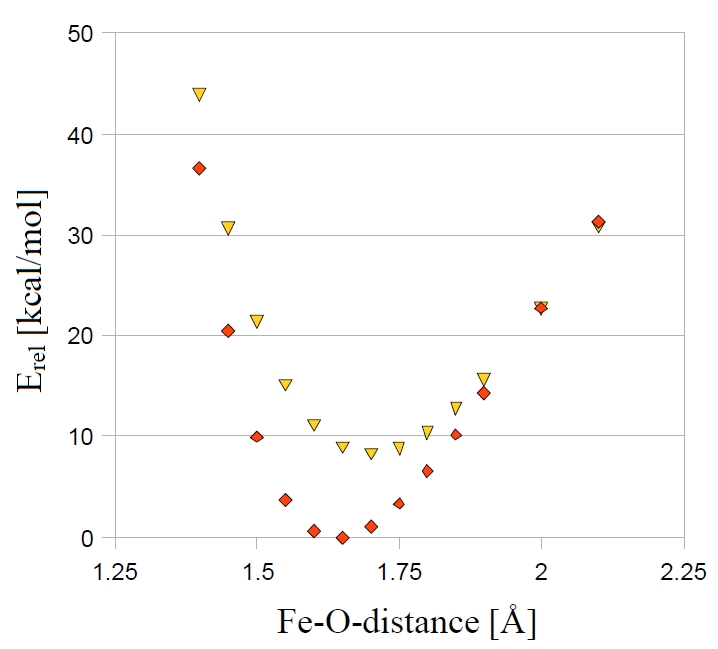
Fig. 6.23 Parameter scan for the quartet and sextet state of [FeO]\(^+\) (B3LYP/SV(P)).
A more realistic example with more than one degree of freedom is the MECP optimization of a structure along the reaction path of the CH\(_{3}\)O \(\leftrightarrow\) CH\(_{2}\)OH isomerization.
!B3LYP SV SurfCrossOpt SurfCrossNumFreq
%mecp Mult 1
  end
*xyz 1 3
 C     0.000000     0.000000     0.000000
 H     0.000000     0.000000     1.300000
 H     1.026719     0.000000    -0.363000
 O    -0.879955     0.000000    -1.088889
 H    -0.119662    -0.866667     0.961546
*
Note
To verify that a stationary point in a MECP optimization is a minimum, you have to use an adapted frequency analysis, called by
SurfCrossNumFreq(see section Minimum Energy Crossing Points).
6.3.13. Conical Intersection Optimization
OBS.: It is currently only available using TD-DFT, will be expanded in future versions. More details about the specific options on Conical Intersections.
A conical intersection (CI) is a complicated 3N-8 dimensional space, where two potential energy surfaces cross and the energy difference between these two states is zero. Inside this so-called “seam-space” minima and transition states can exist. Locating these minima is essential to understand photo-chemical processes, that are governed by non-adiabatic events, as e.g. photoisomerization, photostability - similar to locating transition states for chemical reactions.
As an example for such an analysis we show the conical intersection optimization of the ground and first excited state of singlet ethylene.
Note
Even though locating the CI of a TD-DFT excited state and the reference state is supported, it is not the recommended way of finding the ground state-excited state CI, because such CIs are not described properly by TD-DFT (in particular, TD-DFT even predicts the wrong dimensionality for the intersection space). Instead, it is advised to use SF-TD-DFT for this purpose, e.g. use the \(T_1\) state as the reference state, and calculate both the \(S_0\) and \(S_1\) states as excited states. (vide infra)
!B3LYP DEF2-SVP CI-OPT
%TDDFT IROOT 1 END
* xyz 0 1
C        0.595560237     -0.010483480     -0.000284187
C       -0.831313750      0.167231832      0.001482505
H       -1.381857976      0.227877089      0.963419721
H        1.265119434      0.874806815      0.006897459
H       -1.382258208      0.243775568     -0.959090898
H        1.027489724     -1.032962768     -0.008829646
*
Tip
You can often use a structure between the optimized structures of both states for your CI-optimization. If this doesn’t work, you might try a scan to get a better initial guess.
The results of the CI-optimization are given in the following output. The energy difference between the ground and excited state is printed as E diff. (CI), being reasonabley close for a conical intersection. For a description of the calculation of the non-adiabatic couplings at this geometry, see section Numerical non-adiabatic coupling matrix elements.
                                    .--------------------.
              ----------------------|Geometry convergence|-------------------------
              Item                value                   Tolerance       Converged
              ---------------------------------------------------------------------
              Energy change       0.0000164283            0.0000050000      NO
              E diff. (CI)        0.0000025162            0.0001000000      YES
              RMS gradient        0.0000068173            0.0001000000      YES
              MAX gradient        0.0000136891            0.0003000000      YES
              RMS step            0.0000358228            0.0020000000      YES
              MAX step            0.0000821130            0.0040000000      YES
              ........................................................
              Max(Bonds)      0.0000      Max(Angles)    0.00
              Max(Dihed)        0.00      Max(Improp)    0.00
              ---------------------------------------------------------------------

              Everything but the energy has converged. However, the energy
              appears to be close enough to convergence to make sure that the
              final evaluation at the new geometry represents the equilibrium energy.
              Convergence will therefore be signaled now


                        ***********************HURRAY********************
                        ***        THE OPTIMIZATION HAS CONVERGED     ***
                        *************************************************


     ---------------------------------------------------------------------------
                            Redundant Internal Coordinates

                             --- Optimized Parameters ---
                               (Angstroem and degrees)

         Definition                    OldVal   dE/dq     Step     FinalVal
     ----------------------------------------------------------------------------
      1. B(C   1,C   0)                1.3254 -0.000005 -0.0000    1.3254
      2. B(H   2,C   1)                1.1270  0.000004 -0.0000    1.1270
      3. B(H   3,C   0)                1.1271 -0.000002  0.0000    1.1271
      4. B(H   4,C   1)                1.1271  0.000000 -0.0000    1.1271
      5. B(H   5,C   0)                1.1271 -0.000002  0.0000    1.1271
      6. A(H   3,C   0,H   5)          106.00  0.000001   -0.00    106.00
      7. A(C   1,C   0,H   5)          126.97 -0.000013    0.00    126.97
      8. A(C   1,C   0,H   3)          127.03  0.000011   -0.00    127.03
      9. A(C   0,C   1,H   4)          127.03  0.000013   -0.00    127.03
      10. A(H   2,C   1,H   4)         106.01  0.000001   -0.00    106.01
      11. A(C   0,C   1,H   2)         126.96 -0.000014    0.00    126.96
      12. D(H   2,C   1,C   0,H   5)    73.60  0.000000   -0.00     73.59
      13. D(H   4,C   1,C   0,H   3)    72.78 -0.000001    0.00     72.78
      14. D(H   4,C   1,C   0,H   5)  -106.81  0.000001   -0.00   -106.82
      15. D(H   2,C   1,C   0,H   3)  -106.82 -0.000002    0.00   -106.81
     ----------------------------------------------------------------------------
                  *******************************************************
                  *** FINAL ENERGY EVALUATION AT THE STATIONARY POINT ***
                  ***               (AFTER   12 CYCLES)               ***
                  *******************************************************
CI minima between excited states In an analogous way, the conical intersection minima between two excited states can be requested by selection both an IROOT and a JROOT, shown below.
!B3LYP DEF2-SVP CI-OPT
%TDDFT IROOT 2
       JROOT 1
       #IROOTMULT TRIPLET would search in the triplet PES
       #SF TRUE would search for the S0-S1 CI from a T1 reference, using SF-TD-DFT
       # (but remember to set the multiplicity as 3 instead of 1)
END
* xyz 0 1
C        0.595560237     -0.010483480     -0.000284187
C       -0.831313750      0.167231832      0.001482505
H       -1.381857976      0.227877089      0.963419721
H        1.265119434      0.874806815      0.006897459
H       -1.382258208      0.243775568     -0.959090898
H        1.027489724     -1.032962768     -0.008829646
*
6.3.14. Constant External Force - Mechanochemistry
Constant external force can be applied on the molecule within the EFEI formalism[719] by pulling on the two defined atoms. To apply the external force, use the POTENTIALS in the geom block. The potential type is C for Constant force, indexes of two atoms (zero-based) and the value of force in nN.
! def2-svp  OPT
%geom
  POTENTIALS
    { C 2 3 4.0 }
  end
end

 * xyz 0 1
O          0.73020       -0.07940       -0.00000
O         -0.73020        0.07940       -0.00000
H          1.21670        0.75630        0.00000
H         -1.21670       -0.75630        0.00000
 *
The results are seen in the output of the SCF procedure, where the total energy already contains the force term.
----------------
TOTAL SCF ENERGY
----------------

Total Energy       :         -150.89704913 Eh           -4106.11746 eV

Components:
Nuclear Repulsion  :           36.90074715 Eh            1004.12038 eV
External potential :           -0.25613618 Eh              -6.96982 eV
Electronic Energy  :         -187.54166010 Eh           -5103.26802 eV
6.3.15. Intrinsic Reaction Coordinate
The Intrinsic Reaction Coordinate (IRC) is a special form of a minimum energy path, connecting a transition state (TS) with its downhill-nearest intermediates. A method determining the IRC is thus useful to determine whether a transition state is directly connected to a given reactant and/or a product.
ORCA features its own implementation of Morokuma and coworkers’ popular method.[412] The IRC method can be simply invoked by adding the IRC keyword as in the following example.
! B3LYP SV(P) TightSCF KDIIS SOSCF Freq IRC
* xyz 0 2
  C  -0.000   0.001   -0.000
  H   1.290   0.005   -0.006
  H  -0.330   1.050   -0.002
  H  -0.252  -0.532   -0.929
  H  -0.286  -0.545    0.911
  O   2.499   0.220    0.065
  H   2.509   1.085    0.525
*
For more information and further options see section Intrinsic Reaction Coordinate.
Note
The same method and basis set as used for optimization and frequency calculation should be used for the IRC run.
The IRC keyword can be requested without, but also together with OptTS, ScanTS, NEB-TS, AnFreq and NumFreq keywords.
In its default settings the IRC code checks whether a Hessian was computed before the IRC run. If that is not the case, and if no Hessian is defined via the %irc block, a new Hessian is computed at the beginning of the IRC run.
A final trajectory (_IRC_Full_trj.xyz) is generated which contains both directions, forward and backward, by starting from one endpoint and going to the other endpoint, visualizing the entire IRC. Forward (_IRC_F_trj.xyz and _IRC_F.xyz) and backward (_IRC_B_trj.xyz and _IRC_B.xyz) trajectories and xyz files contain the IRC and the last geometry of that respective run.
6.3.16. Printing Hessian in Internal Coordinates
When a Hessian is available, it can be printed out in redundant internal coordinates as in the following example:
! opt
%geom inhess read
      inhessname "h2o.hess"
      PrintInternalHess true
end
*xyz 0 1
  O      0.000000    0.000000    0.000000
  H      0.968700    0.000000    0.000000
  H     -0.233013    0.940258    0.000000
*
Note
The Hessian in internal coordinates is (for the input
printHess.inp) stored in the fileprintHess_internal.hess.The corresponding lists of redundant internals is stored in
printHess.opt.Although the
!Optkeyword is necessary, an optimization is not carried out. ORCA exits after storing the Hessian in internal coordinates.
6.3.17. Using model Hessian from previous calculations
If you had a geometry optimization interrupted, or for some reason want
to use the model Hessian updated from a previous calculation, you can do
that by passing a basename.opt file, a basename.carthess file or the
initial Hessian on a new calculation.
%GEOM InHess     READ
      InHessName "basename.carthess"
END
6.3.18. Geometry Optimizations using the L-BFGS optimizer
Optimizations using the L-BFGS optimizer are done in Cartesian coordinates. They can be invoked quite simple as in the following example:
! L-Opt
! MM
%mm
  ORCAFFFILENAME "CHMH.ORCAFF.prms"
end
*pdbfile 0 1 CHMH.pdb
Using this optimizer systems with 100s of thousands of atoms can be optimized. Of course, the energy and gradient calculations should not become the bottleneck for such calculations, thus MM or QM/MM methods should be used for such large systems.
The default maximum number of iterations is 200, and can be increased as follows:
! L-Opt
%geom
  maxIter 500 # default 200
 end
*pdbfile 0 1 CHMH.pdb
Only the hydrogen positions can be optimized with the following command:
! L-OptH
But also other elements can be exclusively optimized with the following command:
! L-OptH
%geom
 OptElement F  # optimize fluorine only when L-OptH is invoked.
               #  Does not work with the regular optimizer.
end
When fragments are defined for the system, each fragment can be optimized differently (similar to the fragment optimization described above). The following options are available:
- FixFrags
Freeze the coordinates of all atoms of the specified fragments.
- RelaxHFrags
Relax the hydrogen atoms of the specified fragments. Default for all atoms if !L-OptH is defined.
- RelaxFrags
Relax all atoms of the specified fragments. Default for all atoms if !L-Opt is defined.
- RigidFrags
Treat each specified fragment as a rigid body, but relax the position and orientation of these rigid bodies.
Note
The fragments have to be defined after the coordinate input.
A more complex example is depicted in the following:
! L-OptH
%mm
  ORCAFFFILENAME "CHMH.ORCAFF.prms"
end
*pdbfile 0 1 CHMH.pdb
%geom
 Frags
  2 {8168:8614} end     # First the fragments need to be defined
  3 {8615:8699} end     #  Note that all other atoms belong to
  4 {8700:8772} end     #  fragment 1 by default
  5 {8773:8791} end     #
 RelaxFrags {2} end     # Fragment 2 is fully relaxed
 RigidFrags {3 4 5} end # Fragments 3, 4 and 5 are treated as rigid bodies each.
end
6.3.19. Nudged Elastic Band Method
The Nudged Elastic Band (NEB) method is used to find a minimum energy path (MEP) connecting given reactant and product state minima on the energy surface. An initial path is generated and represented by a discrete set of configurations of the atoms, referred to as images of the system. The number of images is specified by the user and has to be large enough to obtain sufficient resolution of the path. The implementation in ORCA is described in detail in the article by Ásgeirsson et. al.[4] and in section Nudged Elastic Band Method along with the input options. The most common use of the NEB method is to find the highest energy saddle point on the potential energy surface specifying the transition state for a given initial and final state. Rigorous convergence to a first order saddle point can be obtained with the climbing image NEB (CI-NEB), where the highest energy image is pushed uphill in energy along the tangent to the path while relaxing downhill in orthogonal directions. Another method for finding a first order saddle point is the NEB-TS which uses the CI-NEB method with a loose tolerance to begin with and then switches over to the OptTS method to converge on the saddle point. This combination can be a good choice for calculations of complex reactions where the ScanTS method fails or where 2D relaxed surface scans are necessary to find a good initial guess structure for the OptTS method. The zoomNEB variants are a good choice in case of very complex transition states with long tails. For more and detailed information on the various NEB variants implemented in ORCA please consult section Nudged Elastic Band Method.
In their simplest form NEB, NEB-CI and NEB-TS only require the reactant and product state configurations (one via the xyz block, and the other one via the keyword neb_end_xyzfile):
!NEB-TS # or !NEB or !NEB-CI or !ZOOM-NEB-TS or !ZOOM-NEB-CI
        # or !Fast-NEB-TS  (corresponds to IDPP-TS defined in the NEB-TS manuscript)
        # or !Loose-NEB-TS (corresponds to default NEB-TS in the NEB-TS manuscript)
%neb
 neb_end_xyzfile "final.xyz"
end
Below is an example of an NEB-TS run involving an intramolecular proton transfer within acetic acid. The simplest input is
!XTB NEB-TS
%neb
 neb_end_xyzfile "final.xyz"
end

*xyz 0 1
C      0.416168     0.038758    -0.014077
C      0.041816     0.011798     1.439610
O      1.524458     0.176600    -0.453888
O     -0.654209    -0.127881    -0.803857
H     -0.391037    -0.126036    -1.737478
H     -0.913438     0.507022     1.585301
H     -0.057787    -1.026455     1.750845
H      0.819515     0.485425     2.030252
*
Where the final.xyz structure contains the corresponding structure with the proton on the other oxygen.
The initial path is reasonable and the CI calculation can be switched on after five NEB iterations.
Starting iterations:

Optim.  Iteration  HEI  E(HEI)-E(0)  max(|Fp|)   RMS(Fp)    dS
Switch-on CI threshold               0.020000
   LBFGS     0      4    0.081017    0.073897   0.018915  3.2882
   LBFGS     1      5    0.070244    0.056668   0.013913  3.2770
   LBFGS     2      5    0.062934    0.038972   0.008763  3.3376
   LBFGS     3      5    0.057358    0.032076   0.006535  3.3950
   LBFGS     4      4    0.053260    0.019015   0.003599  3.4826

Image  4 will be converted to a climbing image in the next iteration (max(|Fp|) < 0.0200)

Optim.  Iteration  CI   E(CI)-E(0)   max(|Fp|)   RMS(Fp)    dS     max(|FCI|)   RMS(FCI)
Convergence thresholds               0.020000   0.010000            0.002000    0.001000
The CI run converges after another couple of iterations:
*********************H U R R A Y*********************
***        THE NEB OPTIMIZATION HAS CONVERGED     ***
*****************************************************
Subsequently a summary of the MEP is printed:
---------------------------------------------------------------
                         PATH SUMMARY
---------------------------------------------------------------
All forces in Eh/Bohr.

Image Dist.(Ang.)    E(Eh)   dE(kcal/mol)  max(|Fp|)  RMS(Fp)
  0     0.000     -14.45993      0.00       0.00011   0.00004
  1     0.426     -14.44891      6.91       0.00092   0.00033
  2     0.652     -14.42864     19.63       0.00084   0.00038
  3     0.805     -14.41132     30.50       0.00075   0.00027
  4     0.932     -14.40562     34.08       0.00057   0.00018 <= CI
  5     1.044     -14.41047     31.03       0.00057   0.00024
  6     1.153     -14.42200     23.80       0.00103   0.00034
  7     1.280     -14.43666     14.60       0.00098   0.00037
  8     1.476     -14.45106      5.56       0.00106   0.00033
  9     1.869     -14.45988      0.03       0.00013   0.00006
Additionally, detailed information on the highest energy image (or the CI) is printed:
---------------------------------------------------------------
               INFORMATION ABOUT SADDLE POINT
---------------------------------------------------------------

Climbing image                            ....  4
Energy                                    ....  -14.40561577 Eh
Max. abs. force                           ....  9.5976e-04 Eh/Bohr

-----------------------------------------
  SADDLE POINT (ANGSTROEM)
-----------------------------------------
C      0.040867     0.007347    -0.497635
C     -0.075595     0.017879     0.979075
O      1.122340     0.126074    -1.145534
O     -0.928470    -0.137946    -1.298318
H      0.165808    -0.021676    -2.055704
H     -0.996979     0.514720     1.271668
H     -0.116377    -1.013504     1.327873
H      0.788406     0.507105     1.418575

-----------------------------------------
  FORCES (Eh/Bohr)
-----------------------------------------
C     -0.000646    -0.000111     0.000086
...

-----------------------------------------
  UNIT TANGENT
-----------------------------------------
C     -0.246569    -0.031821    -0.019359
...

 => Unit tangent is an approximation to the TS mode at the saddle point

Next a TS optimization is performed on the CI from the NEB run.
Finally, a TS optimization is started, after which the MEP information is updated by including the TS structure:
---------------------------------------------------------------
                      PATH SUMMARY FOR NEB-TS
---------------------------------------------------------------
All forces in Eh/Bohr. Global forces for TS.

Image     E(Eh)   dE(kcal/mol)  max(|Fp|)  RMS(Fp)
  0     -14.45993     0.00       0.00011   0.00004
  1     -14.44891     6.91       0.00092   0.00033
  2     -14.42864    19.63       0.00084   0.00038
  3     -14.41132    30.50       0.00075   0.00027
  4     -14.40562    34.08       0.00057   0.00018 <= CI
 TS     -14.40562    34.08       0.00033   0.00013 <= TS
  5     -14.41047    31.03       0.00057   0.00024
  6     -14.42200    23.80       0.00103   0.00034
  7     -14.43666    14.60       0.00098   0.00037
  8     -14.45106     5.56       0.00106   0.00033
  9     -14.45988     0.03       0.00013   0.00006
Note that here both TS and CI are printed for comparison.