7.18. Interface to POLY_ANISO module
7.18.1. General description
The POLY_ANISO is a stand-alone utility allowing for a semi-ab
initio description of the (low-lying) electronic structure and magnetic
properties of polynuclear compounds. The model behind it is based on the
localised nature of the magnetic orbitals (i.e. the \(d\) and \(f\)
orbitals containing unpaired electrons). For many compounds of interest,
the localised character of the magnetic orbitals leads to very weak
character of the exchange interaction between magnetic centers. Due to
this weakness of the inter-site interaction, the molecular orbitals and
corresponding localised ground and excited states may be optimized in
the absence of the magnetic interaction at all. For this purpose,
various fragmentation models may be applied. The most commonly used
fragmentation model is exemplified in Fig. 7.5:
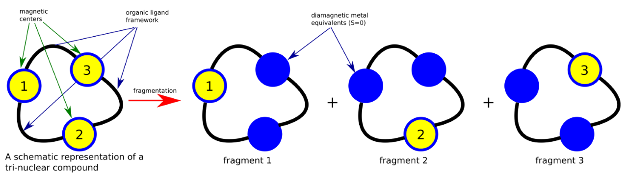
Fig. 7.5 Fragmentation model of a polynuclear compound.
The upper scheme shows a schematic overview of a tri-nuclear compound
and the resulting three mononuclear fragments obtained by diamagnetic
atom substitution method. By this scheme, the neighbouring magnetic
centers, containing unpaired electrons are computationally replaced by
their diamagnetic equivalents. As example, transition metal (TM) sites
are best described by either a diamagnetic Zn(II) or Sc(III), in
function of which one is the closest (in terms of charge and atomic
radius). For lanthanides (LN), the same principle is applicable,
La(III), Lu(III) or Y(III) are best suited to replace a given magnetic
lanthanide. Individual mononuclear metal fragments are then investigated
by the common CASSCF+SOC/NEVPT2+ SOC/SINGLE_ANISO
computational method. A single datafile for each magnetic site,
produced by the SINGLE_ANISO run, is needed by the POLY_ANISO code
as input.
Magnetic interaction between metal sites is very important for accurate
description of low-lying states and their properties. While the full
exchange interaction is quite complex (e.g. requiring a multipolar
description employing a large set of
parameters [413, 871]), in a simplified model it can be
viewed as a sum of various interaction mechanisms: magnetic exchange,
dipole-dipole interaction, antisymmetric exchange, etc. In the
POLY_ANISO code we have implemented several mechanisms, which can be
invoked simultaneously for each interacting pair.
The description of the magnetic exchange interaction is done within the Lines model[527]. This model is exact in three cases:
interaction between two isotropic spins (Heisenberg),
interaction between one Ising spin (only S\(_Z\) component) and one isotropic (i.e. usual) spin, and
interaction between two Ising spins.
In all other cases when magnetic sites have intermediate anisotropy (i.e. when the spin-orbit coupling and crystal field effects are of comparable strengths), the Lines model represents an approximation. However, it was successfully applied for a wide variety of polynuclear compounds so far.
In addition to the magnetic exchange, magnetic dipole-dipole interaction
can be accounted exactly, by using the ab initio computed magnetic
moment for each metal site (as available inside the datafile). In the
case of strongly anisotropic lanthanide compounds (like Ho\(^{3+}\) or
Dy\(^{3+}\)), the magnetic dipole-dipole interaction is usually the
dominant one. For example, a system containing two magnetic dipoles
\(\vec{\mu}_{1}\) and \(\vec{\mu}_{2}\), separated by distance
\(\vec{\textit{r} }\) have a total energy:
where \(\vec{\mu}_{1,2}\) are the magnetic moments of sites 1 and 2, respectively; \(r\) is the distance between the two magnetic dipoles, \(\vec{n}_{1,2}\) is the directional vector connecting the two magnetic dipoles (of unit length). \(\mu_{Bohr}^2\) is the square of the Bohr magneton; with an approximate value of 0.43297 in \(cm^{-1}\)/T. As inferred from the above Equation, the dipolar magnetic interaction depends on the distance and on the angle between the magnetic moments on magnetic centers. Therefore, the Cartesian coordinates of all non-equivalent magnetic centers must be provided in the input.
In brief, the POLY_ANISO is performing the following operations:
read the input and information from the datafiles
build the exchange coupled basis
compute the magnetic exchange, magnetic dipole-dipole, and other magnetic Hamiltonians using the ab initio-computed spin and orbital momenta of individual magnetic sites and the input parameters
sum up all the magnetic interaction Hamiltonians and diagonalise the total interaction Hamiltonian
rewrite the spin and magnetic moment in the exchange-coupled eigenstates basis
use the obtained spin and magnetic momenta for the computation of the magnetic properties of entire poly-nuclear compound
The actual values of the inter-site magnetic exchange could be derived from e.g. broken-symmetry DFT calculations. Alternatively, they could be regarded as fitting parameters, while their approximate values could be extracted by minimising the standard deviation between measured and calculated magnetic data.
7.18.2. Files
POLY_ANISO is called independently of ORCA for now. In the future
versions of ORCA we will aim for a deeper integration, for a better
experience.
bash:$
bash:$  $ORCA/x86_64/otool_poly_aniso  <  poly_aniso.input   >  poly_aniso.output
bash:$
The actual names of the poly_aniso.input and poly_aniso.output are
not hard coded, and can take any names. A bash script for a more
convenient usage of POLY_ANISO can be provided upon request or made
available on the Forum.
7.18.2.1. Input files
The program POLY_ANISO needs the following files:
aniso_i.inputThis is an ASCII text file generated by the
CASSCF/SOC/SINGLE_ANISOrun. It should be provided forPOLY_ANISOasaniso_i.input(i=1,2,3, etc.): one file for each magnetic center. In cases when the entire polynuclear cluster or molecule has exact point group symmetry, onlyaniso_i.inputfiles for crystallographically non-equivalent centers should be given. This saves computational time since equivalent metal sites do not need to be computed ab initio.poly_aniso.inputThe standard input file defining the computed system and various input parameters. This file can take any name.
7.18.2.2. Output files
7.18.3. List of keywords
This section describes the keywords used to control the POLY_ANISO
input file. Only two keywords NNEQ, PAIR (and SYMM if the
polynuclear cluster has symmetry) are mandatory for a minimal execution
of the program, while the other keywords allow customisation of the
execution of the POLY_ANISO.
The format of the “poly_aniso.input” file resembles to a certain extent
the input file for SINGLE_ANISO program. The input file must start
with “&POLY_ANISO” text.
7.18.3.1. Mandatory keywords defining the calculation
Keywords defining the polynuclear cluster:
NNEQ This keyword defines several important parameters of the
calculation. On the first line after the keyword the program reads 2
values: 1) the number of types of different magnetic centers (NON-EQ) of
the cluster and 2) a letter T or F in the second position of the
same line. The number of NON-EQ is the total number of magnetic centers
of the cluster which cannot be related by point group symmetry. In the
second position the answer to the question: “Have all NON-EQ centers
been computed ab initio?” is given: T for True and F for False. On the
following line the program will read NON-EQ values specifying the number
of equivalent centers of each type. On the following line the program
will read NON-EQ integer numbers specifying the number of low-lying
spin-orbit functions from each center forming the local exchange basis.
Some examples valid for situations where all sites have been computed ab initio (case T, True):
NNEQ
  2  T
  1  2
  2  2
There are two kinds of magnetic centers in the cluster; both have been
computed ab initio; the cluster consists of 3 magnetic centers: one
center of the first kind and two centers of the second kind. From each
center we take into the exchange coupling only the ground doublet. As a
result, the \(N_{exch}=2^{1}\times2^{2}=8\), and the two datafiles
aniso_1.input (for-type 1) and aniso_2.input (for-type 2) files must
be present.
NNEQ
  3  T
  2  1  1
  4  2  3
There are three kinds of magnetic centers in the cluster; all three have
been computed ab initio; the cluster consists of four magnetic
centers: two centers of the first kind, one center of the second kind
and one center of the third kind. From each of the centers of the first
kind we take into exchange coupling four spin-orbit states, two states
from the second kind and three states from the third center. As a result
the \(N_{exch}=4^{2}\times2^{1}\times3^{1}=96\). Three files
aniso_i.input for each center (\(i=1,2,3\)) must be present.
NNEQ
  6  T
  1  1  1  1  1  1
  2  4  3  5  2  2
There are six kinds of magnetic centers in the cluster; all six have
been computed ab initio; the cluster consists of 6 magnetic centers:
one center of each kind. From the center of the first kind we take into
exchange coupling two spin-orbit states, four states from the second
center, three states from the third center, five states from the fourth
center and two states from the fifth and sixth centers. As a result the
\(N_{exch}=2^1\times4^{1}\times3^{1}\times5^{1}\times2^{1}\times2^{1}=480\).
Six files aniso_i.input for each center (\(i=1,2,...,6\)) must be
present.
Only in cases when some centers have NOT been computed ab initio (i.e.
for which no aniso_i.input file exists), the program will read an
additional line consisting of NON-EQ letters (\(A\) or \(B\)) specifying the
type of each of the NON-EQ centers: \(A\) - the center is computed ab
initio and \(B\) - the center is considered isotropic. On the following
number-of-B-centers line(s) the isotropic \(g\) factors of the center(s)
defined as \(B\) are read. The spin of the B center(s) is defined:
\(S=(N-1)/2\), where \(N\) is the corresponding number of states to be taken
into the exchange coupling for this particular center. Some examples
valid for mixed situations: the system consists of centers computed ab
initio and isotropic centers (case \(F\), False):
NNEQ
  2  F
  1  2
  2  2
  A  B
  2.3   2.3   2.3
There are two kinds of magnetic centers in the cluster; the center of
the first type has been computed ab initio, while the centers of the
second type are considered isotropic with \(g_X=g_Y=g_Z\)=2.3; the cluster
consists of three magnetic centers: one center of the first kind and two
centers of the second kind. Only the ground doublet state from each
center is considered for the exchange coupling. As a result the
\(N_{exch}=2^1\times2^2=8\). File aniso_i.input (for-type 1) must be
present.
NNEQ
  3  F
  2  1  1
  4  2  3
  A  B  B
  2.3  2.3  2.0
  2.0  2.0  2.5
There are three kinds of magnetic centers in the cluster; the first
center type has been computed ab initio, while the centers of the
second and third types are considered empirically with
\(g_X=g_Y=\)2.3; \(g_Z\)=2.0 (second type) and
\(g_X=g_Y=\)2.0; \(g_Z\)=2.5 (third type); the cluster
consists of four magnetic centers: two centers of the first kind, one
center of the second kind and one center of the third kind. From each of
the centers of the first kind, four spin-orbit states are considered for
the exchange coupling, two states from the second kind and three states
from the center of the third kind. As a result the
\(N_{exch}=4^{2}\times2^{1}\times3^{1}=96\). The file aniso_i.input must
be present.
NNEQ
  6  T
  1  1  1  1  1  1
  2  4  3  5  2  2
  B  B  A  A  B  A
  2.12  2.12  2.12
  2.43  2.43  2.43
  2.00  2.00  2.00
There are six kinds of magnetic centers in the cluster; only three
centers have been computed ab initio, while the other three centers
are considered isotropic; the \(g\) factors of the first center is 2.12
(S=1/2); of the second center 2.43 (S=3/2); of the fifth center 2.00
(S=1/2); the entire cluster consists of six magnetic centers: one center
of each kind. From the center of the first kind, two spin-orbit states
are considered in the exchange coupling, four states from the second
center, three states from the third center, five states from the fourth
center and two states from the fifth and sixth centers. As a result the
\(N_{exch}=2^{1}\times4^{1}\times3^{1}\times5^{1}\times2^{1}\times2^{1}=480\).
Three files aniso_3.input and aniso_4.input and aniso_6.input must
be present.
There is no maximal value for NNEQ, although the calculation becomes
quite heavy in case the number of exchange functions is large.
SYMM Specifies rotation matrices to symmetry equivalent sites. This
keyword is mandatory in the case more centers of a given type are
present in the calculation. This keyword is mandatory when the
calculated polynuclear compound has exact crystallographic point group
symmetry. In other words, when the number of equivalent centers of any
kind \(i\) is larger than 1, this keyword must be employed. Here the
rotation matrices from the one center to all the other of the same type
are declared. On the following line the program will read the number 1
followed on the next lines by as many \(3\times3\) rotation matrices as
the total number of equivalent centers of type 1. Then the rotation
matrices of centers of type 2, 3 and so on, follow in the same format.
When the rotation matrices contain irrational numbers (e.g.
\(\sin\frac{\pi}{6}=\frac{\sqrt{3} }{2}\)), then more digits than
presented in the examples below are advised to be given:
\(\frac{\sqrt{3} }{2}=0.8660254\). Examples:
NNEQ
  2  F
  1  2
  2  2
  A  B
  2.3  2.3  2.3
  SYMM
  1
  1.0 0.0 0.0
  0.0 1.0 0.0
  0.0 0.0 1.0
  2
  1.0 0.0 0.0
  0.0 1.0 0.0
  0.0 0.0 1.0
 -1.0 0.0 0.0
  0.0 -1.0 0.0
  0.0 0.0 -1.0
The cluster computed here is a tri-nuclear compound, with one center computed ab initio, while the other two centers, related to each other by inversion, are considered isotropic with \(g_X=g_Y=g_Z=2.3\). The rotation matrix for the first center is \(I\) (identity, unity) since the center is unique. For the centers of type 2, there are two matrices \(3\times3\) since we have two centers in the cluster. The rotation matrix of the first center of type 2 is Identity while the rotation matrix for the equivalent center of type 2 is the inversion matrix.
NNEQ
  3  F
  2  1  1
  4  2  3
  A  B  B
  2.1 2.1 2.1
  2.0 2.0 2.0
  SYMM
  1
  1.0 0.0 0.0
  0.0 1.0 0.0
  0.0 0.0 1.0
  0.0 -1.0 0.0
  -1.0 0.0 0.0
  0.0 0.0 1.0
  2
  1.0 0.0 0.0
  0.0 1.0 0.0
  0.0 0.0 1.0
  3
  1.0 0.0 0.0
  0.0 1.0 0.0
  0.0 0.0 1.0
In this input a tetranuclear compound is defined, all centers are
computed ab initio. There are two centers of type “1”, related one to
each other by \(C_2\) symmetry around the Cartesian Z axis. Therefore the
SYMM keyword is mandatory. There are two matrices for centers of type
1, and one matrix (identity) for the centers of type 2 and type 3.
NNEQ
  6  F
  1  1  1  1  1  1
  2  4  3  5  2  2
  B  B  A  A  B  A
  2.12 2.12 2.12
  2.43 2.43 2.43
  2.00 2.00 2.00
In this case the computed system has no symmetry. Therefore, the SYMM
keyword is not required. End of Input Specifies the end of the input
file. No keywords after this one will be processed.
7.18.3.2. Keywords defining the magnetic exchange interactions
This section defines the keywords used to set up the interacting pairs of magnetic centers and the corresponding exchange interactions.
A few words about the numbering of the magnetic centers of the cluster
in the POLY_ANISO. First all equivalent centers of the type 1 are
numbered, then all equivalent centers of the type 2, etc. These labels
of the magnetic centers are used further for the declaration of the
magnetic coupling.
PAIRorLIN1This keyword defines the interacting pairs of magnetic centers and the corresponding exchange interaction. A few words about the numbering of the magnetic centers of the cluster in the
POLY_ANISO. First all equivalent centers of the type 1 are numbered, then all equivalent centers of the type 2, etc. These labels of the magnetic centers are used now for the declaration of the magnetic coupling. Interaction Hamiltonian is:\[\hat{H}_{Lines} = -\sum_{p=1}^{N_{pairs} } J_{p}\hat{s}_{i}\hat{s}_{j},\]where \(i\) an \(j\) are the indices of the metal sites of the interacting pair \(p\); \(J_{p}\) is the user-defined magnetic exchange interaction between the corresponding metal sites; \(\hat{s}_{i}\) and \(\hat{s}_{j}\) are the
ab initiospin operators for the low-lying exchange eigenstates.PAIR 3 1 2 -0.2 1 3 -0.2 2 3 0.4
The input above is applicable for a tri-nuclear molecule. Two interactions are antiferromagnetic while ferromagnetic interaction is given for the last interacting pair.
LIN3This keyword defines a more involved exchange interaction, where the user is allowed to define 3 parameters for each interacting pair. The interaction Hamiltonian is given by:
\[\hat{H}_{Lines} = -\sum_{p=1}^{N_{pairs} } \sum_{\alpha} J_{p,\alpha}\hat{s}_{i,\alpha}\hat{s}_{j,\alpha},\]where the \(\alpha\) defines the Cartesian axis \(x,y,z\).
LIN3
1
1 2 -0.2 -0.4 -0.6 # i, j, Jx, Jy, Jz
The input above is applicable for a mononuclear molecule.
LIN9This keyword defines a more involved exchange interaction, where the user is allowed to define 9 parameters for each interacting pair. The interaction Hamiltonian is given by:
\[\hat{H}_{Lines} = -\sum_{p=1}^{N_{pairs} } \sum_{\alpha,\beta} J_{p,\alpha,\beta} \hat{s}_{i,\alpha}\hat{s}_{j,\beta},\]where the \(\alpha\) and \(\beta\) defines the Cartesian axis \(x,y,z\).
LIN9
1
1 2 -0.1 -0.2 -0.3 -0.4 -0.5 -0.6 -0.7 -0.8 -0.9
# i,j,Jxx,Jxy,Jxz,Jyx,Jyy,Jyz,Jzx,Jzy,Jzz
The input above is applicable for a mononuclear molecule.
COORThe
COORkeyword turns ON the computation of the dipolar coupling for those interacting pairs which were declared underPAIR,LIN3orLIN9keywords. On the NON-EQ lines following the keyword the program will read the symmetrised Cartesian coordinates of NON-EQ magnetic centers: one set of symmetrised Cartesian coordinates for each type of magnetic centers of the system. The symmetrized Cartesian coordinates are obtained by translating the original coordinates to the origin of Coordinate system, such that by applying the corresponding SYMM rotation matrix onto the input COOR data, the position of all other sites are generated.COOR 6.489149 3.745763 1.669546 5.372478 5.225861 0.505625
The magnetic dipole-dipole Hamiltonian is computed as follows:
\[\hat{H}_{dip} = \mu_{Bohr}^2 \sum_{p=1}^{N_{pairs}} \frac{ \hat{\mu}_{i}\hat{\mu}_{j} -3(\hat{\mu}_{i} \vec{n}_{i,j} ) (\hat{\mu}_{j} \vec{n}_{i,j})} { \vec{r_{i,j}^{3}}}\]and is added to \(\hat{H}_{exch}\) computed using other models. The \(\hat{H}_{dip}\) is added for all magnetic pairs.
7.18.3.3. Optional general keywords to control the input
Normally POLY_ANISO runs without specifying any of the following
keywords. However, some properties are only computed if it is requested
by the respective keyword. Argument(s) to the keyword are always
supplied on the next line of the input file.
MLTPThe number of molecular multiplets (i.e. groups of spin-orbital eigenstates) for which \(g\), \(D\) and higher magnetic tensors will be calculated (default
MLTP=1). The program reads two lines: the first is the number of multiplets (\(N_{MULT}\)) and the second the array of \(N_{MULT}\) numbers specifying the dimension (multiplicity) of each multiplet. Example:MLTP 10 2 4 4 2 2 2 2 2 2 2
POLY_ANISOwill compute the EPR \(g\) and \(D\)- tensors for 10 groups of states. The groups 1 and 4-10 are doublets (\(\tilde{S} = |1/2\rangle\)), while the groups 2 and 3 are quadruplets, having the effective spin \(\tilde{S} = |3/2\rangle\). For the latter cases, the ZFS (D-) tensors will be computed. We note here that large degeneracies are quite common for exchange coupled systems, and the data for this keyword can only be rendered after the inspection of the exchange spectra.TINTSpecifies the temperature points for the evaluation of the magnetic susceptibility. The program will read three numbers: \(T_{min}\), \(T_{max}\), and \(nT\).
\(T_{min}\) - the minimal temperature (Default 0.0 K)
\(T_{max}\) - the maximal temperature (Default 300.0 K)
\(nT\) - number of temperature points (Default 301)
Example:
TINT
0.0 300.0 331
POLY_ANISOwill compute temperature dependence of the magnetic susceptibility in 331 points evenly distributed in temperature interval: 0.0 K - 330.0 K.HINTSpecifies the field points for the evaluation of the molar magnetisation. The program will read three numbers: \(H_{min}\), \(H_{max}\), \(nH\).
\(H_{min}\) - the minimal field (Default 0.0 T)
\(H_{max}\) - the maximal filed (Default 10.0 T)
\(nH\) - number of field points (Default 101)
Example:
HINT
0.0 20.0 201
POLY_ANISOwill compute the molar magnetisation in 201 points evenly distributed in field interval: 0.0 T - 20.0 T.TMAGSpecifies the temperature(s) at which the field-dependent magnetisation is calculated. Default is one temperature point, T = 2.0 K.
Example:
TMAG
6   1.8 2.0 2.4 2.8 3.2 4.5
ENCUThe keyword expects to read two integer numbers. The two parameters (
NKandMG) are used to define the cut-off energy for the lowest states for which Zeeman interaction is taken into account exactly. The contribution to the magnetisation coming from states that are higher in energy than \(E\) (see below) is done by second order perturbation theory. The program will read two integer numbers: \(NK\) and \(MG\). Default values are: \(NK=100, MG=100\).\[E=NK \cdot k_{Boltz} \cdot \texttt{TMAG}_{max} + MG \cdot \mu_{Bohr} \cdot H_{max}\]The field-dependent magnetisation is calculated at the maximal temperature value given by
TMAGkeyword. Example:ENCU 250 150
If \(H_{max}\) = 10 T and
TMAG= 1.8 K, then the cut-off energy is:\[E=250 \cdot k_{Boltz} \cdot 1.8 + 150 \cdot \mu_{Bohr} \cdot 10 = 1013.06258 (cm^{-1})\]This means that the magnetisation arising from all exchange states with energy lower than \(E = 1013.06258 (cm^{-1})\) will be computed exactly (i.e. are included in the exact Zeeman diagonalisation) The keywords
NCUT,ERATandENCUhave similar purpose. If two of them are used at the same time, the following priority is defined:NCUT > ENCU > ERAT.UBARWith
UBARset to “true”, the blocking barrier of a single-molecule magnet is estimated. The default is not to compute it. The method prints transition matrix elements of the magnetic moment according to the Figure below: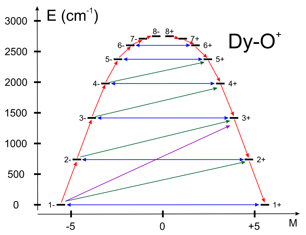
In this figure, a qualitative performance picture of the investigated single-molecular magnet is estimated by the strengths of the transition matrix elements of the magnetic moment connecting states with opposite magnetisations (\(n+ \rightarrow n-\)). The height of the barrier is qualitatively estimated by the energy at which the matrix element (\(n+ \rightarrow n-\)) is large enough to induce significant tunnelling splitting at usual magnetic fields (internal) present in the magnetic crystals (0.01-0.1 Tesla). For the above example, the blocking barrier closes at the state (\(8+ \rightarrow 8-\)). All transition matrix elements of the magnetic moment are given as \(((|\mu_X|+|\mu_Y|+|\mu_Z|)/3)\). The data is given in Bohr magnetons (\(\mu_{Bohr}\)). Example:
UBAR
ERATThis flag is used to define the cut-off energy for the low-lying exchange-coupled states for which Zeeman interaction is taken into account exactly. The program will read one single real number specifying the ratio of the energy states which are included in the exact Zeeman Hamiltonian. As example, a value of 0.5 means that the lowest half of the energy states included in the spin-orbit calculation are used for exact Zeeman diagonalisation. Example:
ERAT
0.333
The keywords
NCUT,ERATandENCUhave similar purpose. If two of them are used at the same time, the following priority is defined:NCUT > ENCU > ERAT.NCUTThis flag is used to define the cut-off energy for the low-lying exchange states for which Zeeman interaction is taken into account exactly. The contribution to the magnetisation arising from states that are higher in energy than lowest \(N_{CUT}\) states, is done by second-order perturbation theory. The program will read one integer number. In case the number is larger than the total number of exchange states(\(N_{exch}\), then the \(N_{CUT}\) is set to \(N_{SS}\) (which means that the molar magnetisation will be computed exactly, using full Zeeman diagonalisation for all field points). The field-dependent magnetisation is calculated at the temperature value(s) defined by
TMAG. Example:NCUT 32
The keywords
NCUT,ERATandENCUhave similar purpose. If two of them are used at the same time, the following priority is defined:NCUT > ENCU > ERAT.MVECMVEC, define a number of directions for which the magnetisation vector will be computed. The directions are given as vectors specifying the direction i of the applied magnetic field).Example:
MVEC
4 # number of directions
1.0 0.0 0.0  # px, py, pz of each direction
0.0 1.0 0.0
0.0 0.0 1.0
1.0 1.0 1.0
ZEEMThis keyword allows to compute Zeeman splitting spectra along certain directions of applied field. Directions of applied field are given as three real number for each direction, specifying the projections along each direction: Example:
ZEEM
6
1.0 0.0 0.0
0.0 1.0 0.0
0.0 0.0 1.0
0.0 1.0 1.0
1.0 0.0 1.0
1.0 1.0 0.0
The above input will request computation of the Zeeman spectra along six directions: Cartesian axes X, Y, Z (directions 1,2 and 3), and between any two Cartesian axes: YZ, XZ and XY, respectively. The program will re-normalise the input vectors according to unity length. In combination with
PLOTkeyword, the correspondingzeeman_energy_xxx.pngimages will be produced.MAVEThe keyword requires two integer numbers, denoted
MAVE_nsymandMAVE_ngrid. The parametersMAVE_nsymandMAVE_ngridspecify the grid density in the computation of powder molar magnetisation. The program uses Lebedev-Laikov distribution of points on the unit sphere. The parameters are integer numbers: \(n_{sym}\) and \(n_{grid}\). The \(n_{sym}\) defines which part of the sphere is used for averaging. It takes one of the three values: 1 (half-sphere), 2 (a quarter of a sphere) or 3 (an octant of the sphere). \(n_{grid}\) takes values from 1 (the smallest grid) till 32 (the largest grid, i.e. the densest). The default is to consider integration over a half-sphere (since \(M(H)=-M(-H)\)): \(n_{sym}=1\) and \(n_{sym}=15\) (i.e 185 points distributed over half-sphere). In case of symmetric compounds, powder magnetisation may be averaged over a smaller part of the sphere, reducing thus the number of points for the integration. The user is responsible to choose the appropriate integration scheme. Note that the program’s default is rather conservative.Example:
MAVE
1  8
TEXPThis keyword allows computation of the magnetic susceptibility \(\chi T(T)\) at experimental points. On the line below the keyword, the number of experimental points \(N_T\) is defined, and on the next \(N_T\) lines the program reads the experimental temperature (in K) and the experimental magnetic susceptibility (in \(cm^{3}Kmol^{-1}\)). The magnetic susceptibility routine will also print the standard deviation from the experiment.
TEXP
54
299.9901   55.27433
290.4001   55.45209
279.7746   55.43682
269.6922   55.41198
259.7195   55.39274
249.7031   55.34379
239.735    55.29292
229.7646   55.23266
219.7354   55.15352
209.7544   55.06556
...
HEXPThis keyword allows computation of the molar magnetisation \(M_{mol}(H)\) at experimental points. On the line below the keyword, the number of experimental points \(N_H\) is defined, and on the next \(N_H\) lines the program reads the experimental field intensity (in Tesla) and the experimental magnetisation (in \(\mu_{Bohr}\)). The magnetisation routine will print the standard deviation from the experiment.
HEXP
3  1.0  5.3  2.4  # temperature values
10 # numer of field points
0.30 4.17 1.26 2.51  # H(T) and M for each temperature
1.00 5.47 3.57 4.82
1.88 5.79 4.54 5.30
2.67 5.92 4.96 5.54
3.46 5.97 5.20 5.70
4.24 6.00 5.36 5.81
5.03 6.01 5.48 5.88
5.82 6.02 5.57 5.93
6.61 6.02 5.65 5.97
7.40 6.03 5.72 5.99
ZJPRThis keyword specifies the value (in \(cm^{-1}\)) of a phenomenological parameter of a mean molecular field acting on the spin of the complex (the average intermolecular exchange constant). It is used in the calculation of all magnetic properties (not for spin Hamiltonians) (Default is 0.0).
ZJPR
-0.02
XFIEThis keyword specifies the value (in T) of applied magnetic field for the computation of magnetic susceptibility by \(dM/dH\) and \(M/H\) formulas. A comparison with the usual formula (in the limit of zero applied field) is provided. (Default is 0.0). Example:
XFIE
0.35
This keyword together with the keyword
PLOTwill enable the generation of two additional plots:XT_with_field_dM_over_dH.pngandXT_with_field_M_over_H.png, one for each of the two above formula used, alongside with respectivegnuplotscripts and gnuplot datafiles.TORQThis keyword specifies the number of angular points for the computation of the magnetisation torque function, \(\vec{\tau}_{\alpha}\) as function of the temperature, field strength and field orientation.
TORQ
55
The torque is computed at all temperature given by
TMAGorHEXP_tempinputs. Three rotations around Cartesian axes X, Y and Z are performed.PRLVThis keyword controls the print level.
2 - normal. (Default)
3 or larger (debug)
PLOTSet to “true”, the program generates a few plots (png or eps format) via an interface to the linux program gnuplot. The interface generates a datafile, a gnuplot script and attempts execution of the script for generation of the image. The plots are generated only if the respective function is invoked. The magnetic susceptibility, molar magnetisation and blocking barrier (
UBAR) plots are generated. The files are named:XT_no_field.dat,XT_no_field.plt,XT_no_field.png,MH.dat,MH.plt,MH.png,BARRIER_TME.dat,BARRIER_ENE.dat,BARRIER.pltandBARRIER.png,zeeman_energy_xxx.pngetc. All files produced bySINGLE_ANISOare referenced in the corresponding output section. Example:PLOT